Mining for alpha with LSTMs
Published January 21, 2024
Time-series classification of daily stock price movements with various memory-aware recurrent models
Intro
As early as 1900, Bachelier presented in Théorie de la spéculation that if speculative prices are indeed fair (i.e. no risk-free expectation of returns), then prices should follow a random walk and are therefore unforecastable (Bachelier (1900)).
In 1970, Fama augmented this argument with emperical research to develop the widely accepted Efficient Market Hypothesis (EMH), which asserts that markets are informationally efficient (Fama (1970)).
In 2004, Timmermann and Granger (2004) point out the self-destructive nature of stable forecasting models, and make the astute observation that model uncertainty comes to the rescue of the semi-strong variant of EMH in the face of successful models, provided that there exists no search technology that reliably identifies these models.
Despite these blows to the prospect of forecasting, recent advancements in compute power and statistical techniques have enabled incredibly powerful seach technologies. Machine Learning applied to price forecasting is a dynamic, growing field, suggesting that models may still be found that are able to exploit non-linear, deeply complex dynamics in market information to yield semi-reliable prediction performance.
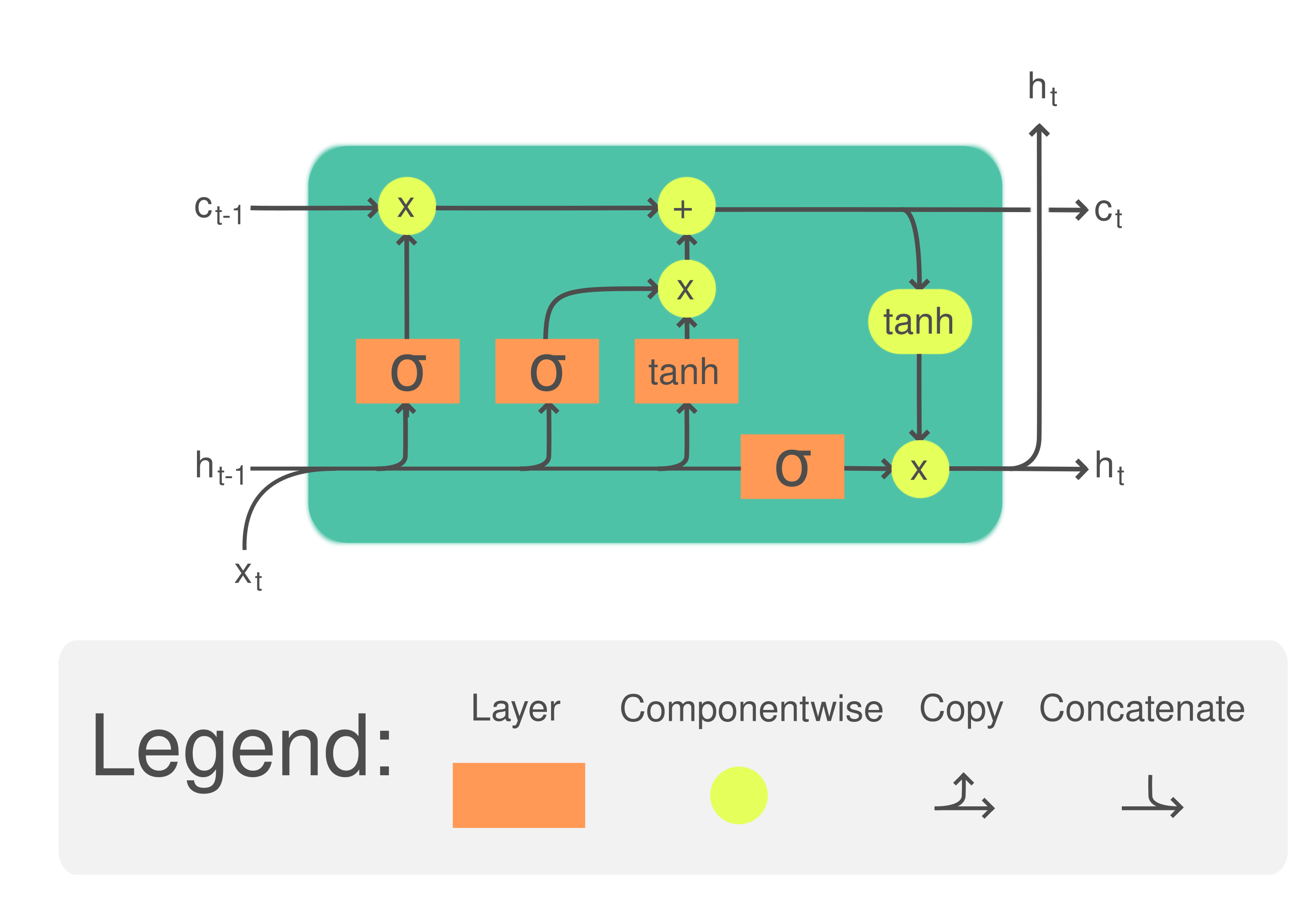
Because traditional deep ANNs treat samples as independent, sequence modeling approaches tend to outperform for the purposes of forecasting (at the expense of training complexity). Popular sequence modeling techniques today make use of Gated Recurrent Units (GRU) and Long-Short Term Memory (LSTM) Neural Networks, which improve upon the lookback capability of Recurrent Neural Networks (RNN) by allowing amplification of influence (memory) of samples farther in the past (Hochreiter and Schmidhuber (1997)).
This essay will briefly discuss the relevant literature before detailing and demonstrating a comprehesive sequence modeling framework built upon the LSTM architecture, and use it to predict short-term stock trend prediction.
The usual disclaimer
It bears repeating that the semi-strong form of market efficiency casts serious doubt on the viability of this type of analysis. Most models in the scientific literature on asset return forecasting problems are trained on publicly-available data. At the end of the day, it’s all still technical analysis, an approach to finance which has extremely weak evidence of efficacy.
What’s more, the techniques used in this essay aren’t particularly sophistocated. LSTMs were introduced in 1997 (Hochreiter and Schmidhuber (1997)), and were undoubtedly deployed by institutional investors shortly thereafter. If a pedestrian LSTM-based architecture can identify inefficiencies in the market, those effects have long since been priced in such that they cannot be systematically exploited.
Relevant literature
Since their introduction in 1997, LSTMs have exploded in popularity in recent years, especially for NLP and forecasting. In the realm of finance, LSTMs have been instrumental in diverse areas ranging from risk management to algorithmic trading, underscoring their adaptability and robustness in handling time-series data.
Many researchers have improved upon the basic LSTM structure, integrating advancements like attention mechanisms and hybrid architectures to enhance prediction accuracy.
Unsurprisingly, researchers (e.g. Shen and Shafiq (2020)1) suggest that beyond model selection and training, feature engineering and selection play a pivotal role in leveraging the full potential of LSTMs in financial applications. This perspective underscores the necessity of domain expertise in financial markets for effective model development.
Wu et al. (2023) presented a more sophistocated use of CNNs and LSTMs to achieve very positive results using a LSTM to compress the information in features of their bespoke SACLSTM framework, achieving high degrees of accuracy for next–day and weekly trend prediction.
Problem statement

The goal of this essay is to compare the performance of RNNs and LSTMs against linear models like AR(p) in predicting price movements for ticker AMZN.
It stands to reason that Small Cap stocks or more niche markets have more inefficiencies in their price data than Mega Caps like AMZN. What’s more, AMZN was highly exposed to macro events like the Dot-com Bubble of the early 2000s and the 2007–2008 financial crisis.
Despite these challenges, results did not improve significantly when testing this model building procedure on Small Cap and less volatile stocks. I did not explore stocks outside of the US market, which may be less efficient.
I therefore define the binary classification problem as follows:
In a given time window, there is typically a non-negligible class imbalance between the two labels. It is unlikely that we can produce a model that accurately classifies 60+% of market movements, so training procedures which do not directly address this imbalance incentivise the models to predict the most frequent label (typically 0). In my training loop, I used a weighted sampling technique to balance the classes.
Data collection and feature engineering
In addition to publicly available OHLC price data, I pulled from several
exogenous sources and constructed several derived covariates. These
included indices, commodity prices, ETFs, risk factors, and macro
indicators. Finally, the library
TA-Lib was
used to expand the features, using the technical analysis cannon (MACD,
Bollinger Bands, etc).
| Data category | Frequency | Imputation technique | Num. feat. |
|---|---|---|---|
| OHLC timeseries (target security, indices, covariate securities) | Daily | linear interpolation | 13 |
| Fama-French 5-factor values | Daily | N/A | 5 |
| Macro indicators | Weekly | resampling + forward-filling | 3 |
Technical indicators (TA-lib) |
Daily | linear interpolation | 312 |
Notable omissions for input features are CDS data, fundamental data, and news (see e.g. Dang et al. (2018)). Other researchers found success by also including options and futures data for the corresponding underlying.
| Feature set | Computation | |
|---|---|---|
| Absolute price level | ||
| Log returns | ||
| Moving average | ||
| Realized volatility |
Feature scaling
ANNs are sensitive to the scaling of input features due to their weighted vector operations and loss optimization algorithms like SGD. There are many popular scaling transformations which work best on certain statistical properties. The input features in the dataset are diverse and therefore have different scaling requirements.
A simple EDA was used to identify patterns in several groups of data. This analysis was done manually and visually; a more comprehensive feature distribution analysis might employ Q-Q plots and stationarity tests like Dickey-Fuller to more accurately and procedurally associate scaling transformers with features.
Figure (3) shows plots of several features from a few categories in table (2).

Note that these categorizations are approximate and only inform the choice of scaling transformer.

Dimensionality reduction (feature selection)
Time dimension:
The timeseries dataset was first reduced along the time dimension. The number of years included in timeseries intended for short-term trend prediction can vary significantly, but is typically around 10 years (Sezer, Gudelek, and Ozbayoglu (2019)).
I therefore truncated the features to between 2003 - 2019, such that a
60-20-20 training-validation-testing split yields around 10 years of
data for training.
Feature dimension:
The number of input features can greatly influence both model accuracy and training performance. The optimal dimensionality reduction technique generates or identifies a small subset of features that is both necessary and sufficient to predict the target. In their paper, Shen and Shafiq (2020) appeared to have positive results with between 10 and 20 features, with diminishing returns for higher feature counts. I found that between 15 and 30 features produced the best results. Though this parameter can be optimized through cross validation, aiming for this range was generally sufficient.

There are many dimensionality reduction techniques on offer for time series. For example, one popular technique is RFE; I’m not sure where this technique first appeared, but e.g. Guyon et al. (2002) used RFE backed by an SVM to identify important genes for use in a cancer classification context.
Another common technique is to train on the principal components of the features, though I remain skeptical that an unsophisticated application of this technique offers significant improvement over a simple collinearity reduction, especially given that PCA is blind to the very temporal structure in the data which our sequence modeling techniques hope to exploit.
Feature importance with Boruta
Boruta feature selection (Kursa and Rudnicki (2010)) is an "all-relevant" feature selection algorithm. The algorithm wraps a Random Forest classifier and works by comparing the relevance of real features to that of random probes. Though Boruta was not originally designed to handle time series, Li et al. (2024) propose Boruta for stock price prediction, followed by various signal processing techniques (denoising) to achieve impressive results.
Because the features have a wide range of statistical properties (see Fig. (2)), a tree-based approach is preferred as an initial filter in the pipeline.
Figure (5) shows the results of an RFC before and after Boruta feature selection. A tree depth of 5 was set for the RFC as recommended by the Boruta python library documentation.

Multi-collinearity analysis
To further eliminate redundant features, I collapse pairwise-correlated features with a threashold of 0.8. .
Note that pairwise correlation is not sufficient to detect all multi-collinearity in the feature space; techniques like Variance Inflation Factor (VIF) can be used for further reduction.

The features left after this elimination step are the final features. The final number of features is 26, just which lies in the target range of 10-30.
Figure (7) shows a multi-scatter plot of the final features and looks promising; the pairwise relationships between the features are somewhat uncorrelated but nonetheless have some interesting structure.

Model selection and training
Data preprocessing
The strength of the models we will be evaluating comes from their ability to amplify and retain information about datapoints in the past. For this reason, data must be shaped appropriately.
Sequence length is a tunable hyperparameter of the data pipeline; however, I chose a static value of 20 trading days across all models. This time horizon is used frequently for short-term trend prediction in the DL forecasting survey (Sezer, Gudelek, and Ozbayoglu (2019)) and is long enough to capture several potential autocorrelation frequencies (day, week, month).
Each input (training example) consists of a
(seq_length, num_features)
tensor. Training and inference used a batch size of 64.
Baseline and memory-aware models
The goal is to evaluate the performance of a deep sequence model backed by an LSTM ANN. To sanity-check the results of the tuned model, we first build up in complexity to the final LSTM architecture.
Table (3) lists some of the classes of models in order of increasing complexity.
| Model class | Description | Approx. num. params |
|---|---|---|
| LogisticMLP-AR(p) | An depth NN with (flattens input to size input_dim * lookback) |
2000-4000 |
| RNN | Vanilla RNNs with 1-3 hidden layers and 8-16 hidden units (varying degrees of dropout). | 400-700 |
| GRU | GRUs with 1-3 hidden layers and 8-12 hidden units (varying degrees of dropout). | 800-3300 |
| LSTM | LSTMs with 1-3 hidden layers and 8-10 hidden units (varying degrees of dropout). | 1700-3300 |
There are many great resources online explaining the architectures of the RNN-based models, though be cautious about tutorials which apply them to financial data. Many presenters make fundamental mistakes (incorrect target definition and data leakage are common offenses).
Optimization
The ADAM optimizer, introduced by Kingma and Ba in 2014 (Kingma and Ba
(2014)), is an updated version of RMSProp that tracks
running averages of gradients and 2nd moments of gradients. All
applicable models used this optimizer with default parameters from
torch.optim.Adam
throughout the training process.
Results
Figure (8) shows
evaluation metrics for a sampling of models on the validation and test
datasets. Arguably, the best performing model was
lstm-1-12-0.2
(single-layer LSTM with 12 hidden units and 0.2 dropout probability),
acheiving an AUC of 0.53; i.e. a 3% improvement on random guessing.
While the LSTM and GRU classes of models outperformed RNNs a majority of
the time, optimal hyperparameters were the most important factor in the
model’s performance. Given a reasonable set of starting parameters,
LSTMs were not guaranteed to outperform their RNN cousins; in fact,
multi-layer LSTMs almost always yielded weaker results than even the
baseline vanilla MLP architectures.
The performance of a subset of models on the validation and test datasets is shown in (8).

The significance of the various metrics shown above ultimately depends on the investor’s strategy. One famous and strikingly simple application of this type of buy-signal generation is for statistical arbitrage, whereby models are trained on several assets in a basket, and long / short positions are taken on assets with the highest / lowest probability for up-moves, respectively (Krauss, Do, and Huck (2017), Fischer and Krauss (2017)). The construction of an optimal trading strategy for a given model behavior is out of scope for this essay, though I may explore it in the future.
Assessing memory effects
In order to assess the presence of memory effects, I construct a simple metric which compares AUC scores of the model when shown the full memory (sequence length) vs. when it is shown only the current day. A similar technique was used by Kraft et. al. to quantify memory effects in their LSTM models for predicting global vegitation states with climate data (Kraft et al. (2019)).
Table (4) shows the metric for some of the models, tested on the out-of-sample test set.
| Model | |
|---|---|
lstm-1-12-0.2 |
-0.0124 |
gru-2-08-0.2 |
0.0037 |
lstm-2-08-0.2 |
0.033 |
The memory effects are quite weak, with some models actually performing worse when given longer context. Statistical tests such as McNemar’s Test or DeLong’s Test for AUC can be used to assess the significance of these results.
Conclusion
In this essay, several common memory-aware Neural Network architectures, RNN, GRU, and LSTM, were trained on public financial data to predict next-day price movements. While the models were able to consistently beat 50-50 guessing, the improvement was marginal, and the presence of memory effects in the models’ weights was weak.
If an investor is to have any hope of constructing a profitable trading strategy around one of the models featured in this esssay, they would require far better performance than I was able to achieve in order to offset transaction costs.
There were several challenges during the training process.
-
The LSTM layers have a large number of parameters which can easily overfit on the
num_feat * seq_lenfeatures. Various dropout percentages were used to mitigate overfitting, though a more optimal strategy should be explored. -
It is expected that there is a low signal-to-noise ratio in the data. Even with weighted sampling, the models tended to settle into local minima by simply predicting 0 most of the time. A more careful feature engineering procedure and deeper hyperparameter search may yield better results, though practitioners should be skeptical of high out-of-sample binary accuracy results.
-
This procedure used a sequential TRAIN-VAL-TEST split of data. Since we are training on daily buy signals, the TRAIN data may have little relevance to the the TEST data, because the two timeframes are separated by several years. A competent trading strategy would readjust model parameters each day.
There are many immediate improvements which can be made to the training procedure, such as better cross validation and the inclusion of more sophistocated factors used in practice by factor investors. Analysis of longer-term trends (e.g. monthly, quarterly) may also yield better results, as the noise found in daily returns is avoided (e.g. Khaidem, Saha, and Dey (2016) achieved accuracy with a Random Forest classifier for 1, 2, and 3 month periods).
References
Bachelier, Louis. 1900. “Théorie de La Spéculation.” Annales Scientifiques de L’Ecole Normale Supérieure 17: 21–88.
Dang, L. Minh, Abolghasem Sadeghi, Huy Huynh, Kyungbok Min, and Hyeonjoon Moon. 2018. “Deep Learning Approach for Short-Term Stock Trends Prediction Based on Two-Stream Gated Recurrent Unit Network.” IEEE Access PP (September): 1–1.
Fama, Eugene F. 1970. “Efficient Capital Markets: A Review of Theory and Empirical Work.” The Journal of Finance 25 (2): 383–417.
Fischer, Thomas, and Christopher Krauss. 2017. “Deep Learning with Long Short-Term Memory Networks for Financial Market Predictions.” FAU Discussion Papers in Economics 11/2017. Friedrich-Alexander University Erlangen-Nuremberg, Institute for Economics.
Guyon, Isabelle, Jason Weston, Stephen Barnhill, and Vladimir Vapnik. 2002. “Gene Selection for Cancer Classification Using Support Vector Machines.” Machine Learning 46 (1): 389–422.
Hochreiter, Sepp, and Jürgen Schmidhuber. 1997. “Long Short-Term Memory.” Neural Computation 9 (8): 1735–80.
Khaidem, Luckyson, Snehanshu Saha, and Sudeepa Roy Dey. 2016. “Predicting the Direction of Stock Market Prices Using Random Forest.”
Kingma, Diederik P., and Jimmy Ba. 2014. “Adam: A Method for Stochastic Optimization.” CoRR abs/1412.6980.
Kraft, Basil, Martin Jung, Marco Körner, Christian Requena Mesa, José Cortés, and Markus Reichstein. 2019. “Identifying Dynamic Memory Effects on Vegetation State Using Recurrent Neural Networks.” Frontiers in Big Data 2.
Krauss, Christopher, Xuan Anh Do, and Nicolas Huck. 2017. “Deep Neural Networks, Gradient-Boosted Trees, Random Forests: Statistical Arbitrage on the s&p 500.” Eur. J. Oper. Res. 259: 689–702.
Kursa, Miron B., and Witold R. Rudnicki. 2010. “Feature Selection with the Boruta Package.” Journal of Statistical Software 36 (11): 1–13.
Li, Jing, Yukun Liu, Hongfang Gong, and Xiaofei Huang. 2024. “Stock Price Series Forecasting Using Multi-Scale Modeling with Boruta Feature Selection and Adaptive Denoising.” Applied Soft Computing 154: 111365. https://doi.org/
Sezer, Omer Berat, Mehmet Ugur Gudelek, and Ahmet Murat Ozbayoglu. 2019. “Financial Time Series Forecasting with Deep Learning : A Systematic Literature Review: 2005-2019.” Papers 1911.13288. CoRR. Vol. abs/1911.13288. arXiv.org.
Shen, Jingyi, and M. Omair Shafiq. 2020. “Short-Term Stock Market Price Trend Prediction Using a Comprehensive Deep Learning System.” Journal of Big Data 7 (1): 66.
Timmermann, Allan, and Clive W. J. Granger. 2004. “Efficient Market Hypothesis and Forecasting.” International Journal of Forecasting 20 (1): 15–27. https://doi.org/
Wu, Jimmy Ming-Tai, Zhongcui Li, Norbert Herencsar, Bay Vo, and Jerry Chun-Wei Lin. 2023. “A Graph-Based CNN-LSTM Stock Price Prediction Algorithm with Leading Indicators.” Multimedia Systems 29 (3): 1751–70.