How Not to Visualize Martingales
Published February 14, 2024
A cautionary tale about the subtleties of stochastic process simulation
TL;DR
While exploring the properties of various continuous-time stochastic processes, I had a bit of fun simulating them in python using discrete approximations generated via the Euler-Maruyama method.
In order to check my work when manipulating various stochastic random variables using Itô calculus, I built a Martingale Detector - a crude tool which tests a drift hypothesis via Monte Carlo methods.
When the naive detection scheme yielded unexpected results for certain processes, I discovered that I had implicitly baked in a faulty assumption in my code.
I believe that the bug described below is an instructive example of the consequences of eschewing rigor when designing simulations. This essay is equal parts mathematical candy and postmortem.
While my use for the tool was rather pedestrian (checking my work on some practice problems), testing for signals like Martingale and Markov properties in stochastic time-series is actually of great interest in fields like finance and physics.
The usual disclaimer: The purpose of this essay is to document my experience and present some food for thought to the reader. The procedures described below should not be relied upon for anything important.
A brief review of Martingales
Assume a filtered probability space is given. An -adapted process is a continuous-time martingale if and only if and
Proving the martingale conditions for simple stochastic processes which can be expressed in closed-form often requires little more than some massaging using the tools of Itô calculus and basic probability theory. For example, for processes which can be expressed as functions of a standard Wiener process and time , it is sufficient to prove
Still, I wanted a quick-and-dirty way to check my work, preferrably with a method that makes few assumptions about the underlying dynamics.
The Naive Martingale Detector
The problem domain
I didn’t bother formalizing requirements for the types of processes which the tool should handle. The general form of stochastic differential equations describes far too broad a domain of processes and admits many pathological examples which could evade any numerical drift detector I throw at it 1.
I essentially restricted and to analytic functions or Itô integrals of analytic functions. I may revisit this topic in the future to further generalize the revised tool presented at the end of this essay.
While fancy non-parametric techniques like bootstrapping might be a more mathematically sound tool for the job, Monte Carlo will essentially give me a population standard deviation estimate () to any degree of precision my CPU can stand, thus making a -test a reasonable choice. CLT, take the wheel!
A better name for this tool might be the Drift Detector 2, since we will be evaluating a Martingale null hypothesis.
Spoiler alert:
The above null is NOT equivalent to invalidating the Martingale property; the nature of this mistake is the primary subject of this essay.
Aiming for simplicity, I ran a -test for each timestep and rejected the null upon discovery of any breaches.
Detection procedure
For the following, let . 3
My naive (indeed faulty!) scheme for drift detection is essentially a series of hypothesis tests driven by Monte Carlo simulation. The details:
-
Sample stochastic increments from a Gaussian4; i.e. .
-
Perform discrete integration of the to obtain , ensuring that .
-
Shift the to the left such that any vectorized operations on and are properly aligned (I may describe this step in further detail later, but it is largely unimportant for this discussion).
-
Construct via Euler-Maruyama. At this point, path realizations of can be rendered to get a sense of their dynamics.
-
Drift detection step: Compute -statistics for each timestep 5 and test the null.
Below are some examples of the detector working as designed.
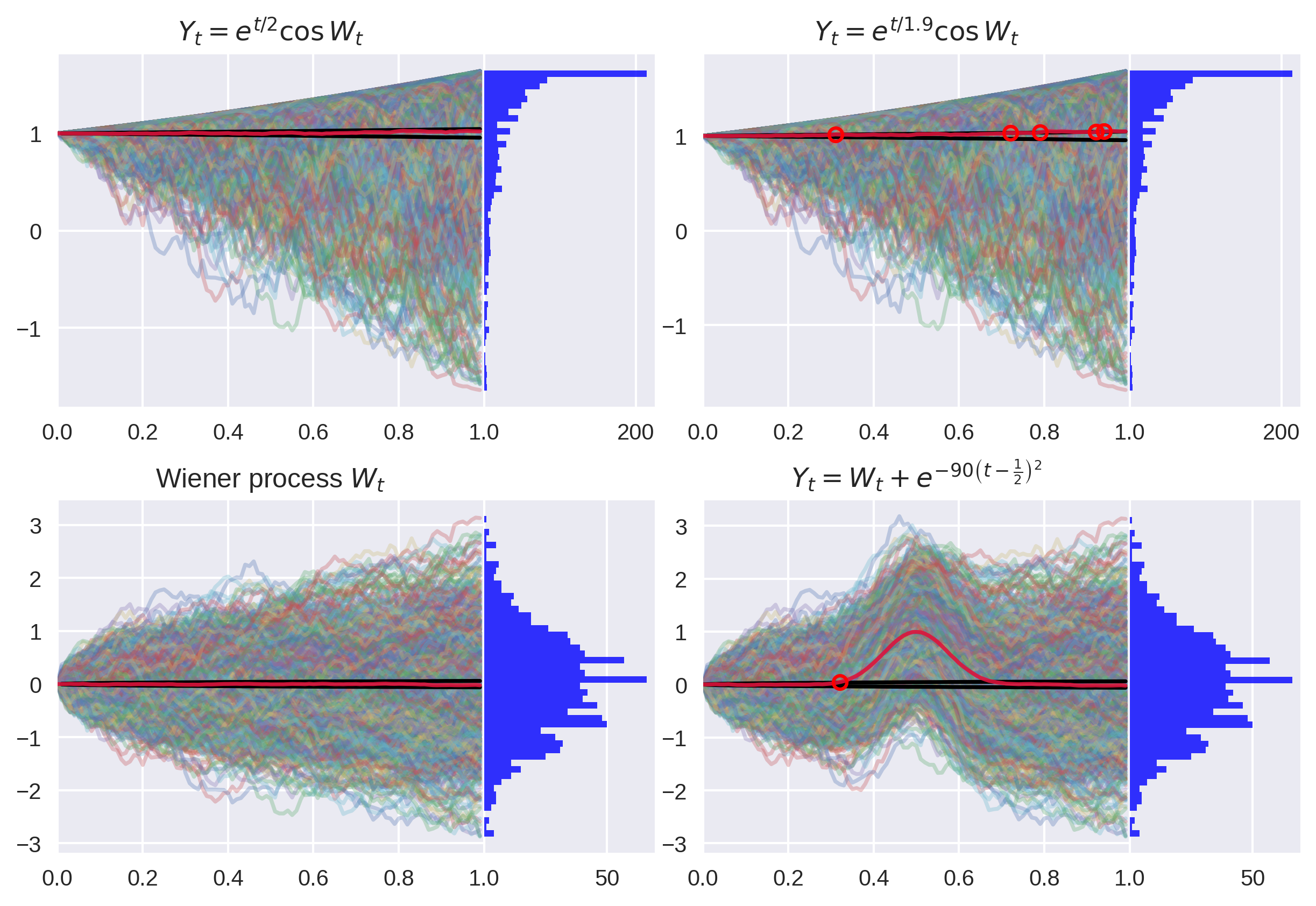
Figure 1: A Monte Carlo path simulation with significance level shown as black lines. The test correctly fails to reject the null for Martingale and correctly rejects the Martingale null for near-Martingale (breaches shown as red circles).
Notice the growing critical region boundaries (in black) as the processes diffuse.
For good measure, I included the Wiener process, which passes unsurprisingly. I also cooked up some more exotic test cases, like processes which are locally driftless at the boundaries of the interval. This test will catch these types of processes, up to the resolution of the discretization.
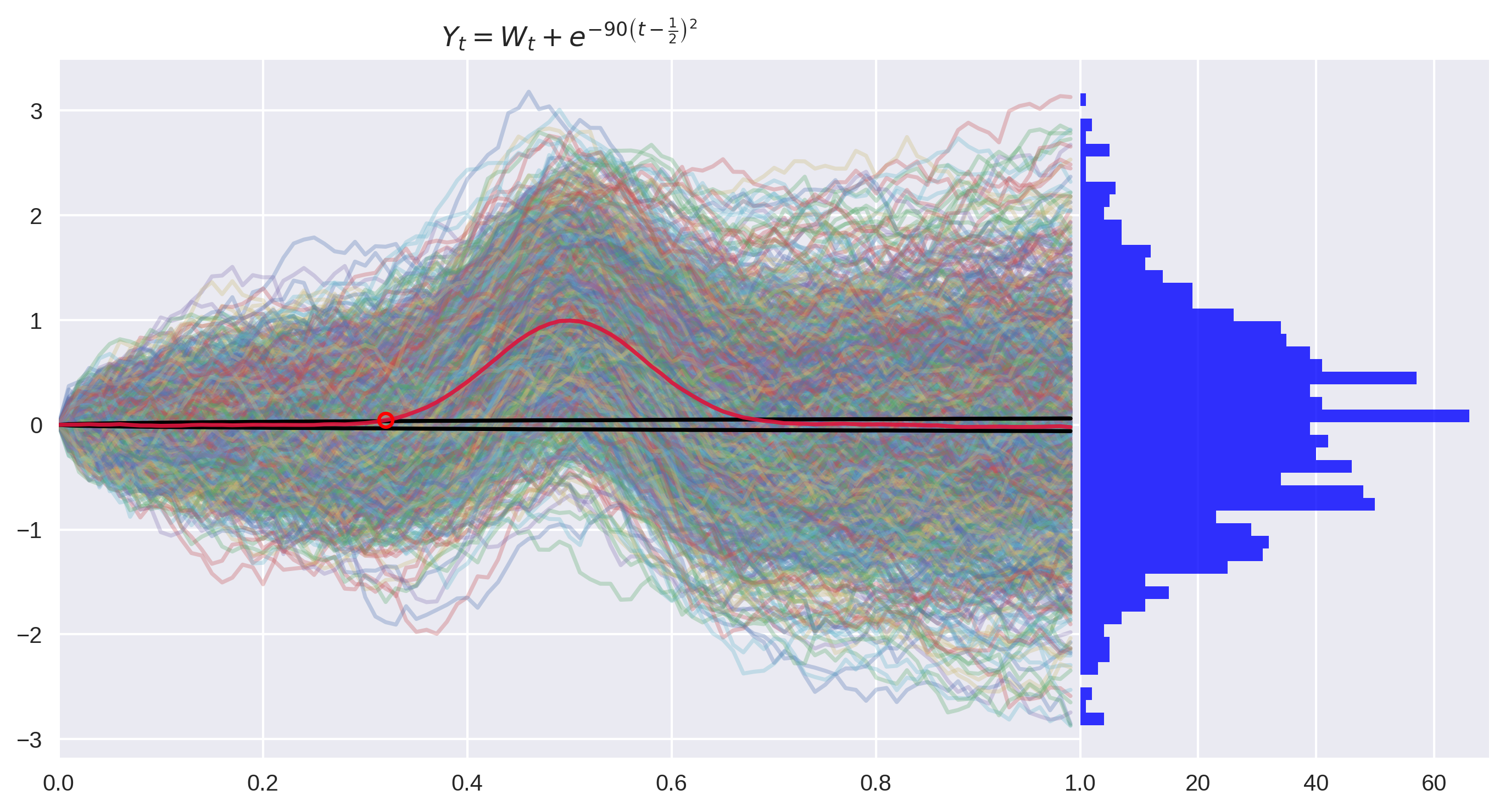
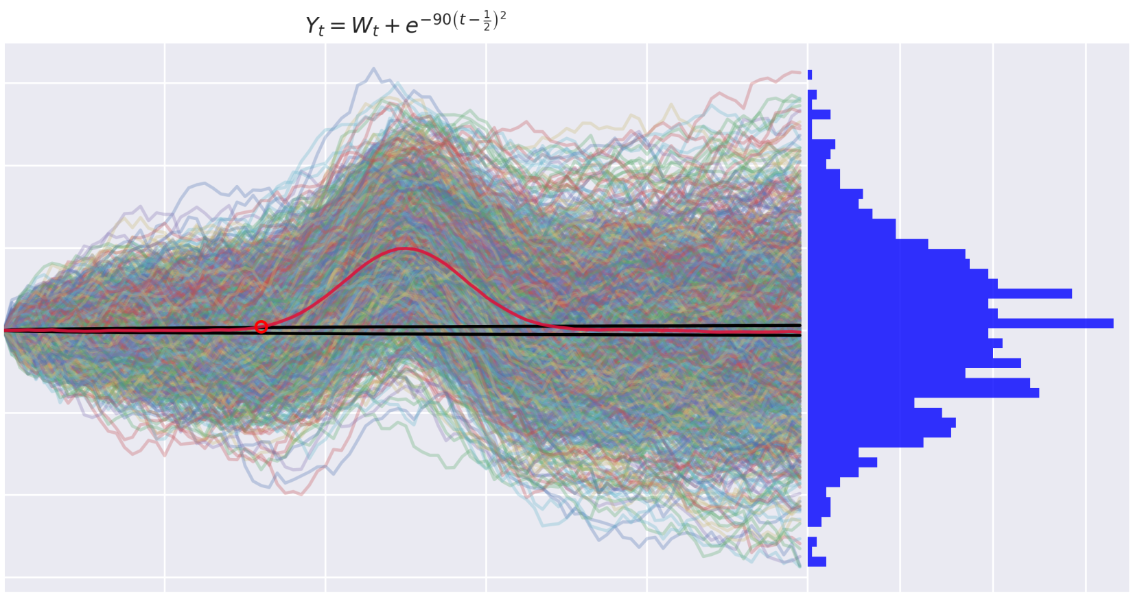
Figure 2: This process satisfies the Martingale properties locally but not globally.
Alas, it was too good to be true!
I quickly noticed the detector making Type 2 errors for certain processes, some of which are shown below.
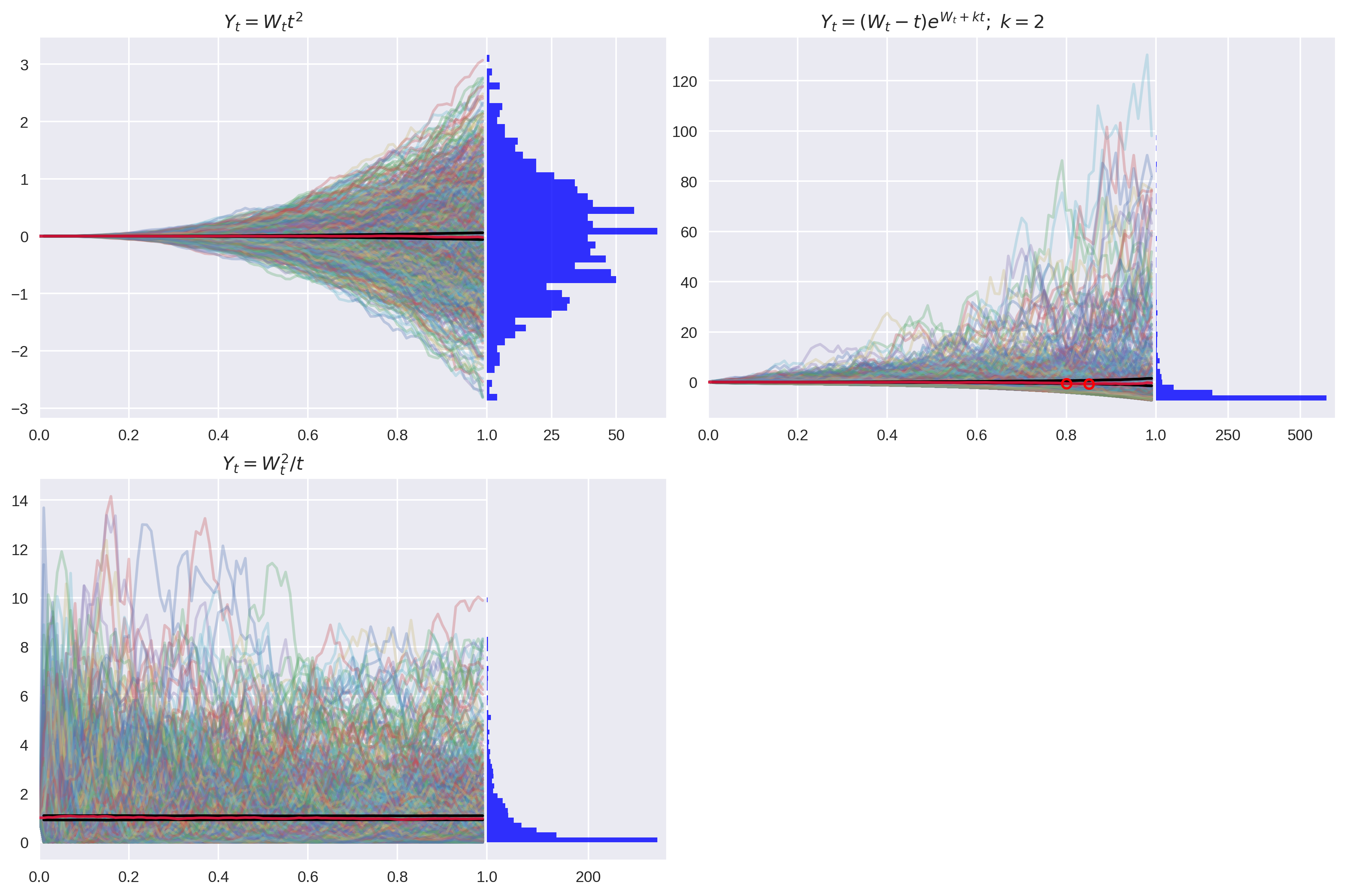
Figure 3: Examples of non-Martingales which caused Type 2 errors in the detector.
In the case of , we do indeed see a few breaches. However, they do not appear on all seeds, and when they do, the -values are very close to the significance level. We will treat this example as a false negative.
I suspect this is a sampling error which is easily resolved by generating more paths. Nevertheless, I have kept this seed in the essay to demonstrate that getting these types of tests right is tricky!
In order to diagnose the problem, we need to analyze the two non-Martingales shown above 6.
-
(correctly identified)
-
(false negative)
I set out to build a tool to sanity-check my math; now we must rely on the math to debug the tool!
Non-Martingale examples
Non-Martingale 1: correctly identified
Consider the process
Then . To proceed further, define . By Itô’s lemma,
This stochastic differential equation is equivalent to the more flexible integral form:
Rearranging,
Finally, have
So is not a martingale for all .
Non-Martingale 2: false negative
Consider the following process:
The conditional expectation is relatively easy to calculate. There may be more elegant methods, but I computed the expectation by brute force, taking advantage of the normality of the quantity .
There are then just two functions of Gaussian quantities for which the expectation must be found. Let
It is trivial to show that
Finally,
So is not a martingale for all .
This bears a striking resemblance to the result for . So why does the martingale detection method work for , but not for ?
So, what went wrong?
The Monte Carlo techniques used by the Naive Martingale Detector work by path averaging, i.e.
where convergence in probability is guaranteed by the Weak Law of Large Numbers.
Spot the mistake? converges on the unconditional expectation of , whereas the martingale property is defined by the expectation of conditional upon the filtrations !
For stochastic processes whose expectation conditioned on is always some static value, the Naive Martingale Detector will "report" a false positive!
The originally proposed null hypothesis is invalid because it implies a conditional expectation only on and no other values. It is not equivalent to the Martingale drift property.
Hopefully it’s clear now why the Naive Martingale Detector failed or succeeded for the processes discussed earlier.
-
The process has unconditional expectation .
NMD correctly identified the drift. -
The process has unconditional expectation .
NMD false negative. -
The process has unconditional expectation .
NMD false negative.
Fixing the Naive Martingale Detector
There are many ways to fix the Naive Martingale Detector. The first is my solution and admittedly a bit hacky; the second is the test used in most papers on this topic.
Solution 1: Mind the filtration
This solution is a bit crude but allows us to keep most of the code from the Naive Martingale Detector.
After implementing this, I was pleased to find that a more refined version of this strategy was used successfully in this paper: Park and Whang (2005)
Modify the hypothesis:
for some and some .
The conditional probability is the key here; there may be many expressions which work. I found a simple threshold filter to yield good results.
The best results are obtained by setting test parameters and manually for each process; luckily, this is not hard to do. A filter at time (about 25% along the axis) works for all processes, but doesn’t always lead to good visuals. At first, I somewhat arbitrarily used but switched to filtering the upper quartile to accommodate processes with highly clustered distributions.
Here, we revisit the false negatives from above, this time armed with the new detector.
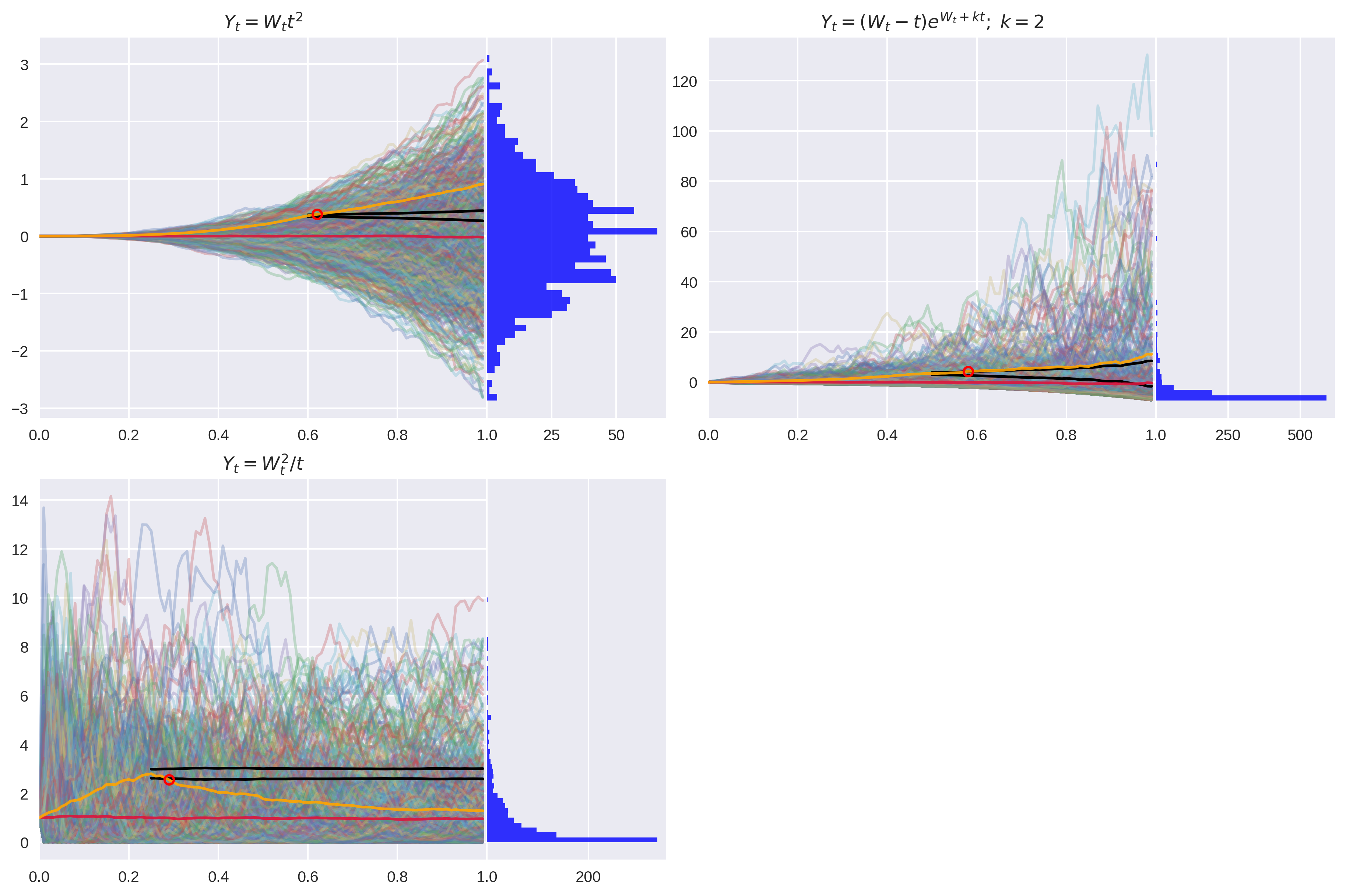
Figure 4: Corrected Detector with unconditional expectation (red) and filtered expectation (orange).
Success! Now, we must ensure there is no regression for the first examples in this essay.
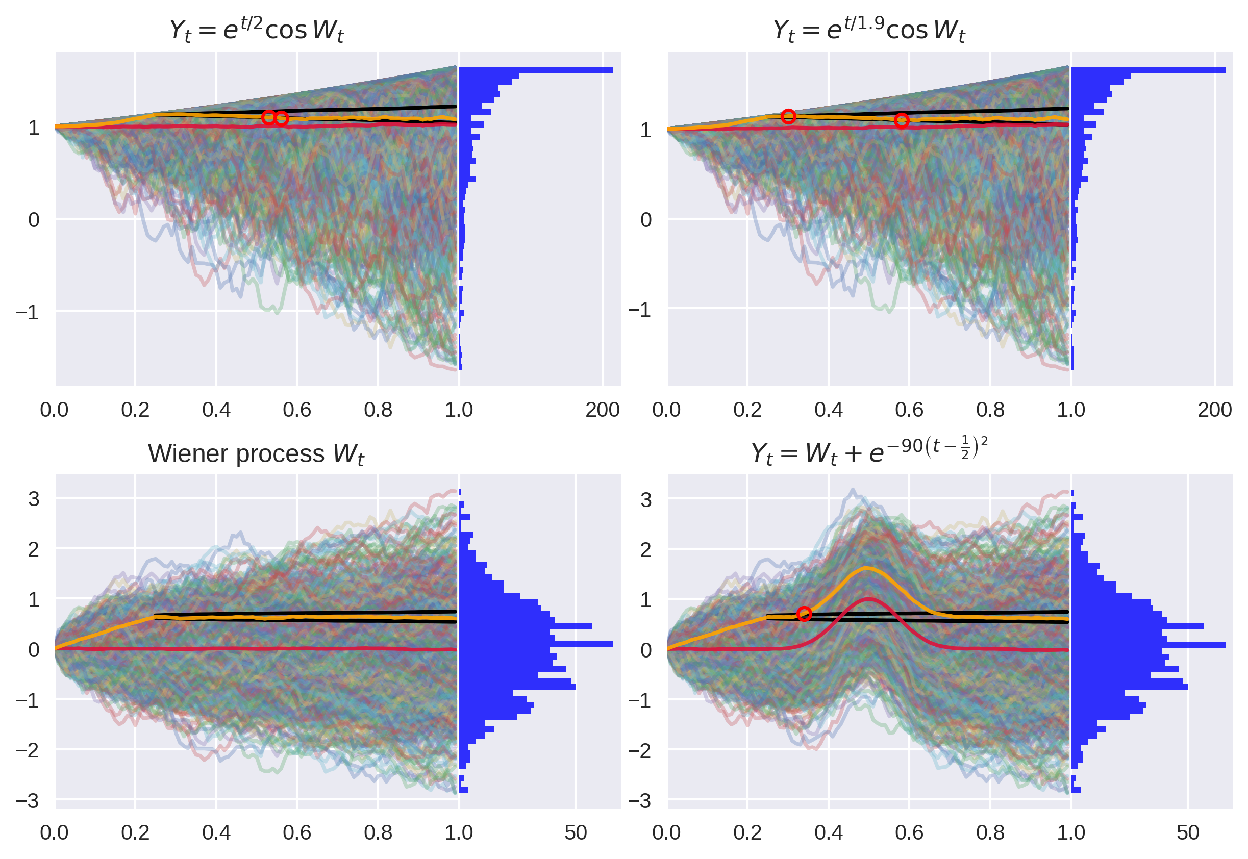
Figure 5: Qualitatively, these Martingales exhibit much less drift after filtering when compared to their non-Martingale cousins above.
Unfortunately, we have indeed regressed here, erroneously rejecting the null hypothesis for the process . On the bright side, it’s not due to a flaw in logic, but it does expose a weakness of this approach. I believe sampling error is the culprit in this instance, since we filter out 75% of the samples before testing. It’s trivial to compensate for this with a larger initial sample size.
I am confident that one could construct a clever process which could systematically break this revised procedure. If you can find one, I’d love to hear about it!
Solution 2: Autoregressive model
Up to this point, every solution discussed (valid or otherwise) just throws CPU power at the problem quite brutishly. This approach is often tempting (and incredibly powerful), especially when time is of the essence.
But I would be doing the reader a great disservice if I did not mention the right way to solve this problem. This approach is not my own; full credit goes to the many people who have contributed to its development.
Instead of analyzing cross-sections of samples, model the sequence and test for the strength of the drift term in an AR(p) model. For AR(1), model
To make this useful, assume a unit root ( = 1) so that
Thus, we have our Martingale null hypothesis:
Clever indeed! For more, see this paper from Phillips and Jin: Phillips and Jin (2014)
Final thoughts
I’d like to document some of my takeaways here, written as advice to my future self.
Just because it works in practice, doesn’t mean it works in theory!
Wikipedia lists the 4 defining properties of the Wiener process . I designed the path generation procedure described in this essay to preserve properties 1, 3, and 4 (obviously sacrificing continuity). The path generation itself worked well.
However, the mere existence of a functioning discretization mechanism should not lead you to assume that some continuous analog of that mechanism even exists, much less is the fundamental engine of the object of study!
For a while, I operated with the mental model that a realization of the Wiener process was constructed by some mysterious mathematical supercomputer running my same algorithm but with an uncountably infinite array of . But of course, this is the wrong mathematical framing! Instead, entire paths (on some interval) are indexed by samples , and we observe the properties of these objects through the -indexed lenses provided by a filtration (a proxy for real-world ignorance) on the underlying probability space.
Notice that appears nowhere in the 4 defining properties of the Wiener process. really comes from Itô calculus 7, when Itô generalized the Riemann-Stieltjes integral to stochastic settings in the 1940s, two decades after Wiener’s formalization.
More lessons: lightning round
-
There is a place for rigor when designing simulations, and it can be rewarding to nail down seemingly abstract mathematical objects.
-
When designing and debugging simulations, be explicit about your assumptions; own and challenge them. Understand what you lose when discretizing.
-
Use caution when switching between mathematical contexts. Brownian motion and its cousins are interesting objects of study because they are fundamentally random and fundamentally continuous.
Simulations always make compromises. But simulations like this have additional (sometimes quite subtle) sources of potential error (e.g. discretization error, sampling error, even accumulating floating point errors).
-
Quality testing of code is critical; focus on edge cases and combinations of edge cases.
References
Park, Joon Y., and Yoon-Jae Whang. 2005. “A Test of the Martingale Hypothesis.” Studies in Nonlinear Dynamics & Econometrics 9 (2): 1–32. https://doi.org/10.2202/1558-3708.1163.
Phillips, Peter C. B., and Sainan Jin. 2014. “Testing the Martingale Hypothesis.” Journal of Business & Economic Statistics 32 (4): 537–54. https://doi.org/10.1080/07350015.2014.908780.
- For example, hide drift at some irrational number that the discretization will miss.↩
- but Martingale Detector is better for branding!↩
- In order to simplify the notation throughout, I often switch between continuous-time and discrete-time notation without much justification. I’ll hand wave here and appeal to the strong convergence of order of Euler-Maruyama; discretization does not play a major role in the arguments herein.↩
- Of course, this need not be a Gaussian so long as the first and second moments are correct!↩
- I’m sure there is some kind of fancy aggregation statistic or early-stopping method which is more optimal, but this worked fine for a first attempt.↩
- I’ve added constants in and ( and ) to make the math more general. As you will see, only particular values of these constants make the processes Martingales, which were not used above.↩
- I’m not sure if stochastic increments appeared before this; the point is that Wiener’s original model did not use them.↩