Building a Model for Returns
Published September 28, 2024

Volatility drag in Gaussian stochastic return models
Who needs anyway?
Quantitative finance follows in the tradition set by Bachelier in his 1900 paper "Théorie de la spéculation" [Bachelier 1900], in which he models asset prices as fundamentally random. In quantitative finance, we throw up our hands and leave the business of trying to forecast prices to the value investors and the day-traders. Once we acquiesce to a nondeterministic universe1, we ask "ok, now what can we do?"
Bachelier essentially started with an arithmetic binomial model and considered the transition probability between timesteps to obtain a stochastic diffusion process:
Into the 60s and 70s, however, a preference emerged to model asset prices as stochastic processes which were geometric, both in drift and diffusion. This is certainly an improvement, but it leads to subtleties which are not present in Bachelier’s arithmetic model.
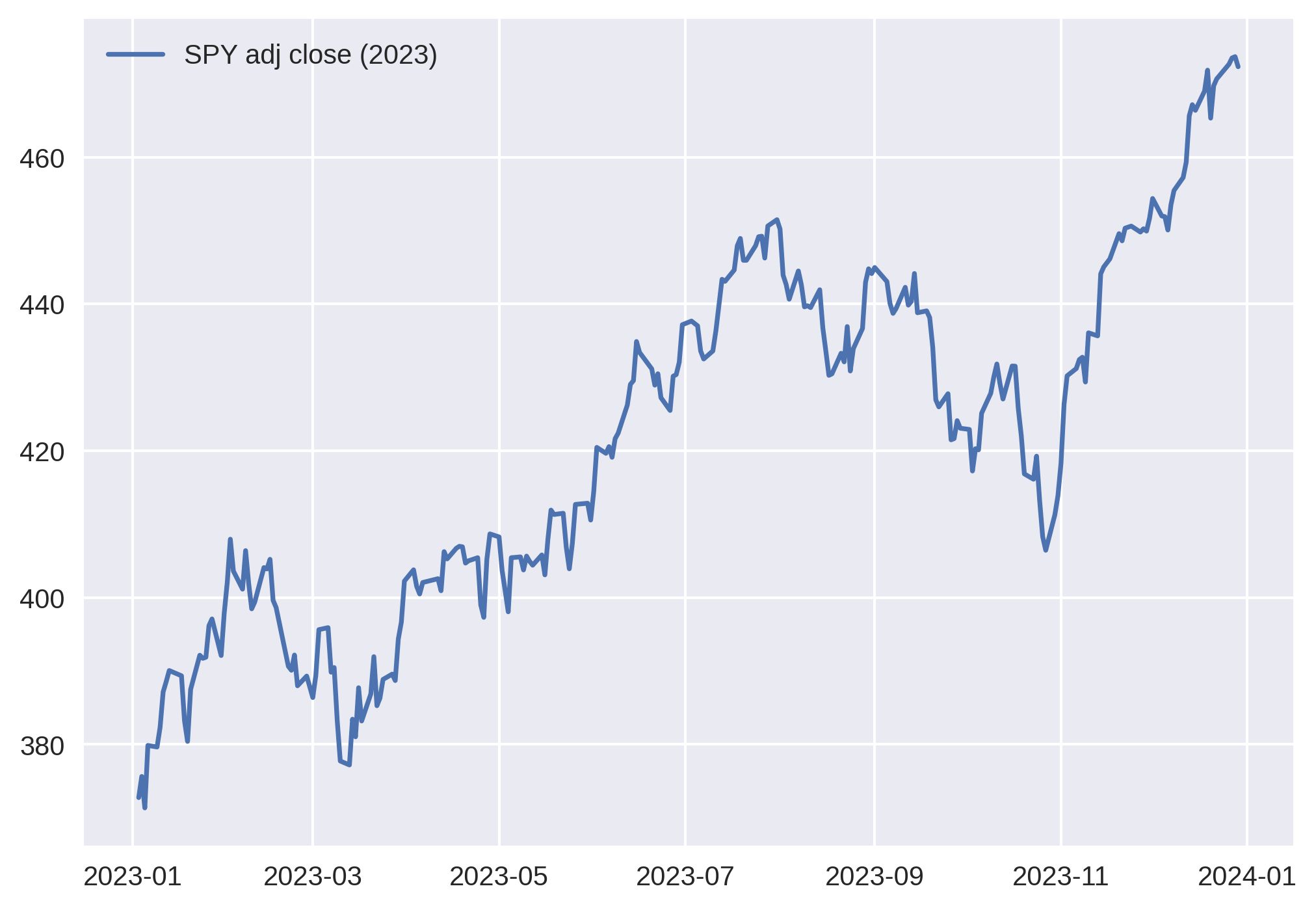
Daily asset price data for SPY is chaotic at every time scale. Fractals, anyone?
We begin by considering a discrete time series indexed by time.
The series describes the stock price at particular times , and crucially, we declare it to be random. In this probabilistic setting proposed by Bachelier, descriptive statistics of some underlying random variable can grant us an initial foothold in describing the jagged, chaotic time series of asset prices. Of course, efficient markets mostly strip these statistics of useful information, but their properties are instructive.
We might consider the entire sequence to be a random variable, i.e. , but it’s not clear how we would extend this definition or sample from its distribution in practice. The individual prices might be another choice, though their distributions clearly depend on the realized previous price (in other words, the amount by which the price can change over a timestep appears bounded). Bachelier considered the sequence of absolute differences to solve this problem, but we can do better.
To proceed, we make an empirical observation.
The average change in over an interval is proportional to and the length of the interval.
This suggests that the stock’s movement has something to do with exponential growth, and it’s why a geometric stochastic process model is a better choice.
A couple important points:
-
It’s important to recognize the above as a purely empirical fact. This is not generally true for an arbitrary sequence of numbers.
-
The noise in real-world market data can make it difficult to convince yourself of this unless you look at sufficiently small intervals across sufficiently large time scales, and I wonder if that’s why Bachelier didn’t bother with this mathematical framing. Across short time scales, with the resolution of price data Bachelier had access to, the relationship would have appeared linear.
-
Even still, the statement is a simplification which does not survive statistical scruitiny. This is a restatement of the classic (over)simplification that is lognormally distributed – this is only an approximation.
This also means that, while studying the properties of the indeed leads to the same answers, the math gets a bit cluttered, as the distribution of depends on . Thus, a natural choice is to reframe the model in terms of the main character of this essay: returns.
Returns are noisy and somewhat Gaussian, and since annual return is simply compounded daily returns, it’s fair to think of the asset price path as "growth plus noise." The subtle interplay of this growth and noise is the subject of this essay.
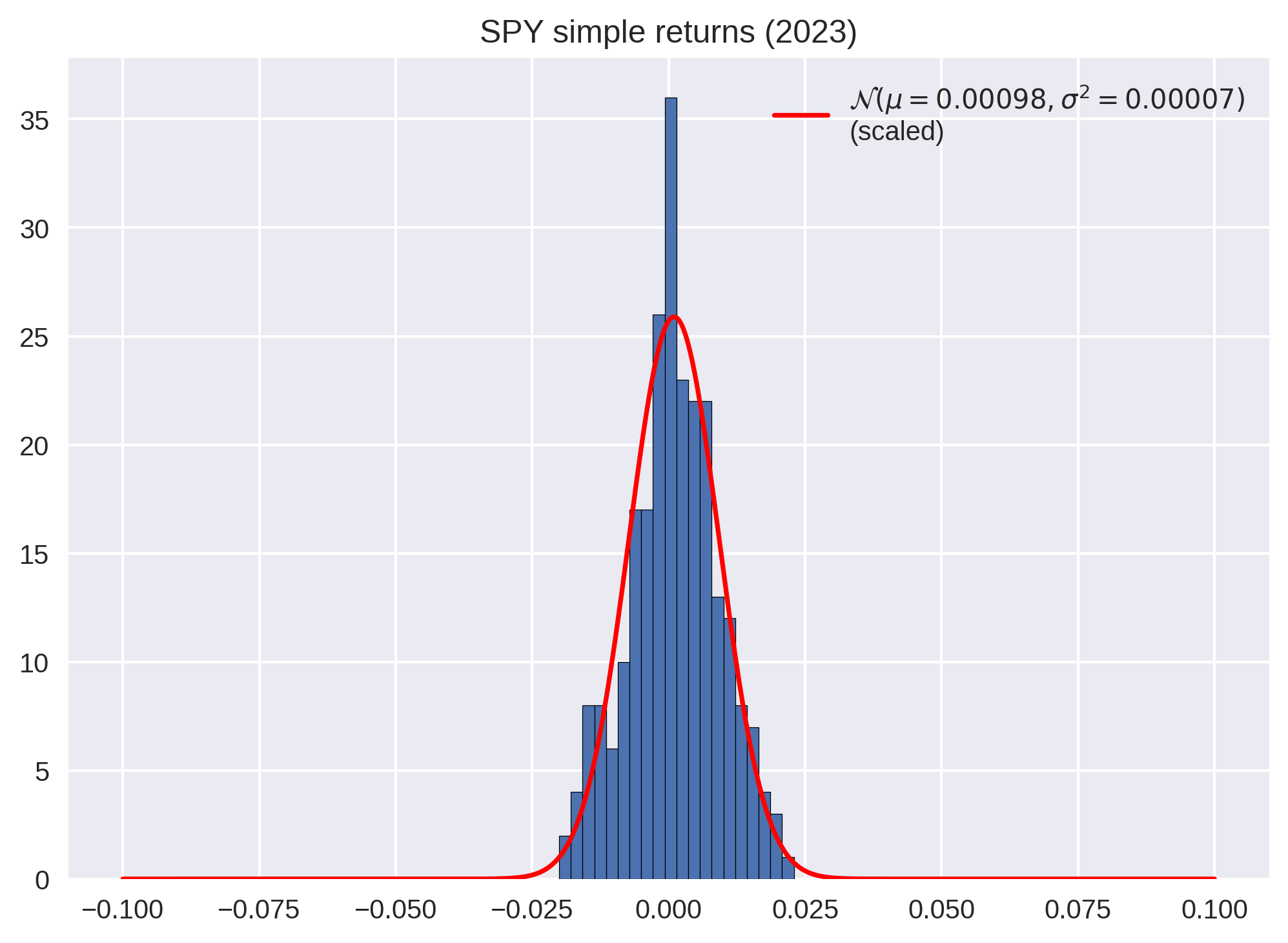
Histogram of simple returns. If you blur your eyes and shake your head back and forth, you might convince yourself that it resembles a Gaussian distribution.
A tale of two growth rates
Let’s start by formalizing our choice of random variable. Emperically, we approximated that
so a natural first step is to model a sequence of simple returns.
Here, I introduce the notation to indicate that this return is defined across a timestep . The notation may seem cumbersome, but it will prove quite useful later on.
But we can eliminate our dependence on another way: by considering log returns.
Under this view, the sequence becomes
The implication of modeling the asset price as random is to claim that it could have ended differently. So what is the event space? Recall the emperical observation from earlier, this time in terms of returns:
We’ll label these proportionality constants and respectively, so that
Now that we have chosen or as the engine of the price sequence, we can reason about the event space. Both approaches have the result of turning the geometric problem into a linear one. Furthermore, we can see that, under our assumptions, and do not depend on time. Thus, if we have a sufficiently large number of returns, we can replace our sample averages with the expectations.
This is a good start, but we have a mystery on our hands. If we think of a stock price as "growth plus noise", which growth rate is the correct one? And what does the other one represent?
The growth rate associated with simple returns might feel more legitimate at first. After all, simple returns are all that really matters in finance – they are the actual amount of money gained or lost.
For kicks, let’s superimpose these growth rates atop the same SPY time series.
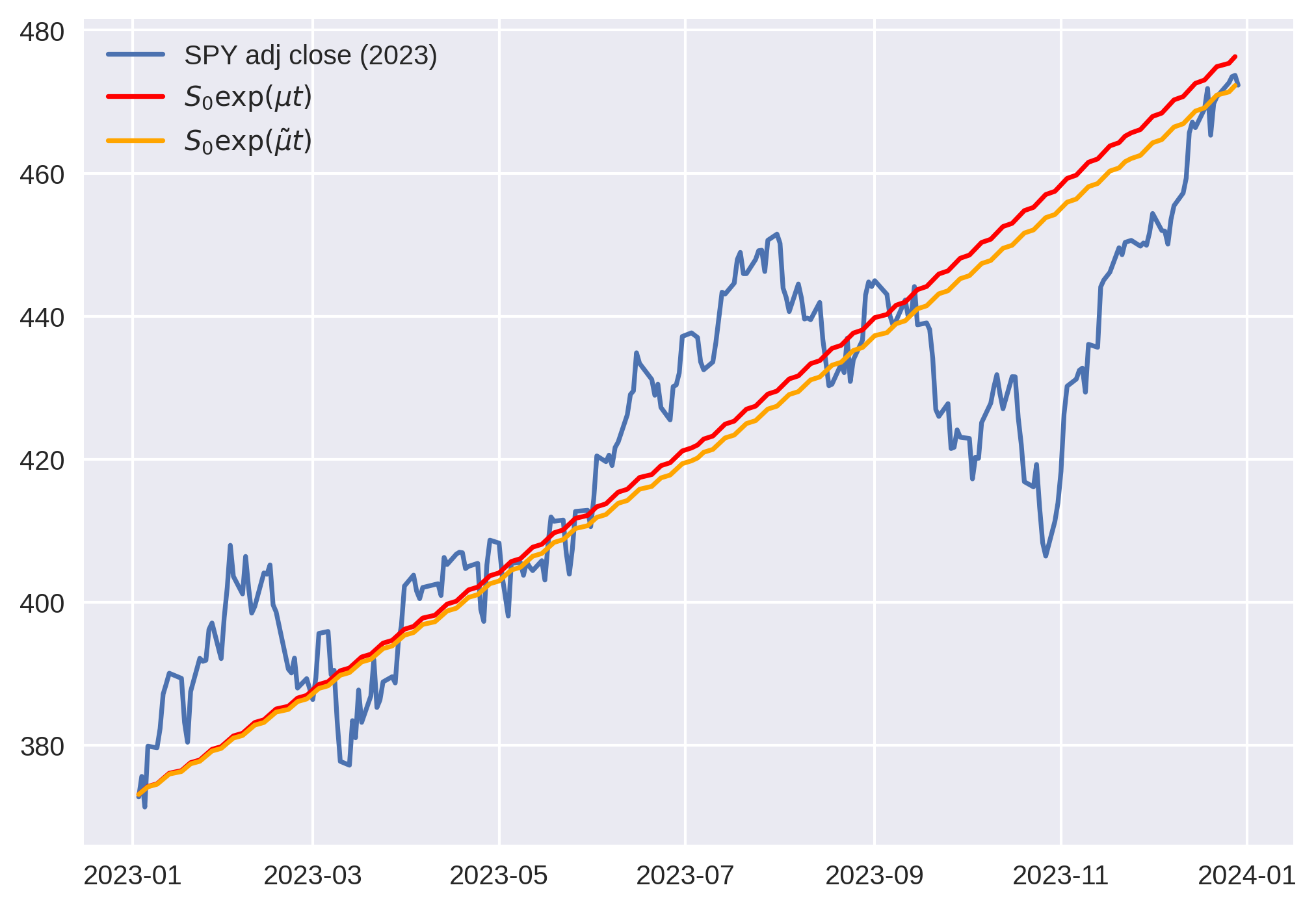
The growth rate obtained from simple returns overestimates total return, whereas mean log returns does not. Note that is small enough that . The base of exponentiation is insignificant; the difference is in the growth rate itself.
In some sense, this view makes seem more legitimate, since it preserves total return! If indeed our stock price is "growth plus noise," surely this growth curve is the ideal deterministic basis with which to compose the noise.
We can rewrite these random variables equivalently as discrete random growth factors (i.e. price ratios).
We can safely ignore terms smaller than . But be careful – we cannot ignore terms of order .
We can see that these price ratio expectations are the arithmetic and geometric means of the price ratios, respectively. The AM-GM inequality tells use that will always be larger than .
This view also explains why log returns recover the total return.
The mean log return simply answers the question "what growth rate, if compounded times, would result in the correct total growth?"
You might not think that this difference is a big deal; for the period of SPY prices shown above, the two differ by only about 3.6%.
But consider pathological cases where these two quantities have different signs. As it turns out, in markets, this happens all the time. I tested 252-day windows for 15 stocks, and for most stocks, a whopping 5% of their year-long windows exhibit this behavior – overall positive daily returns but with a negative total return! This should convince you that understanding the difference between these two growth rates is worthwhile.
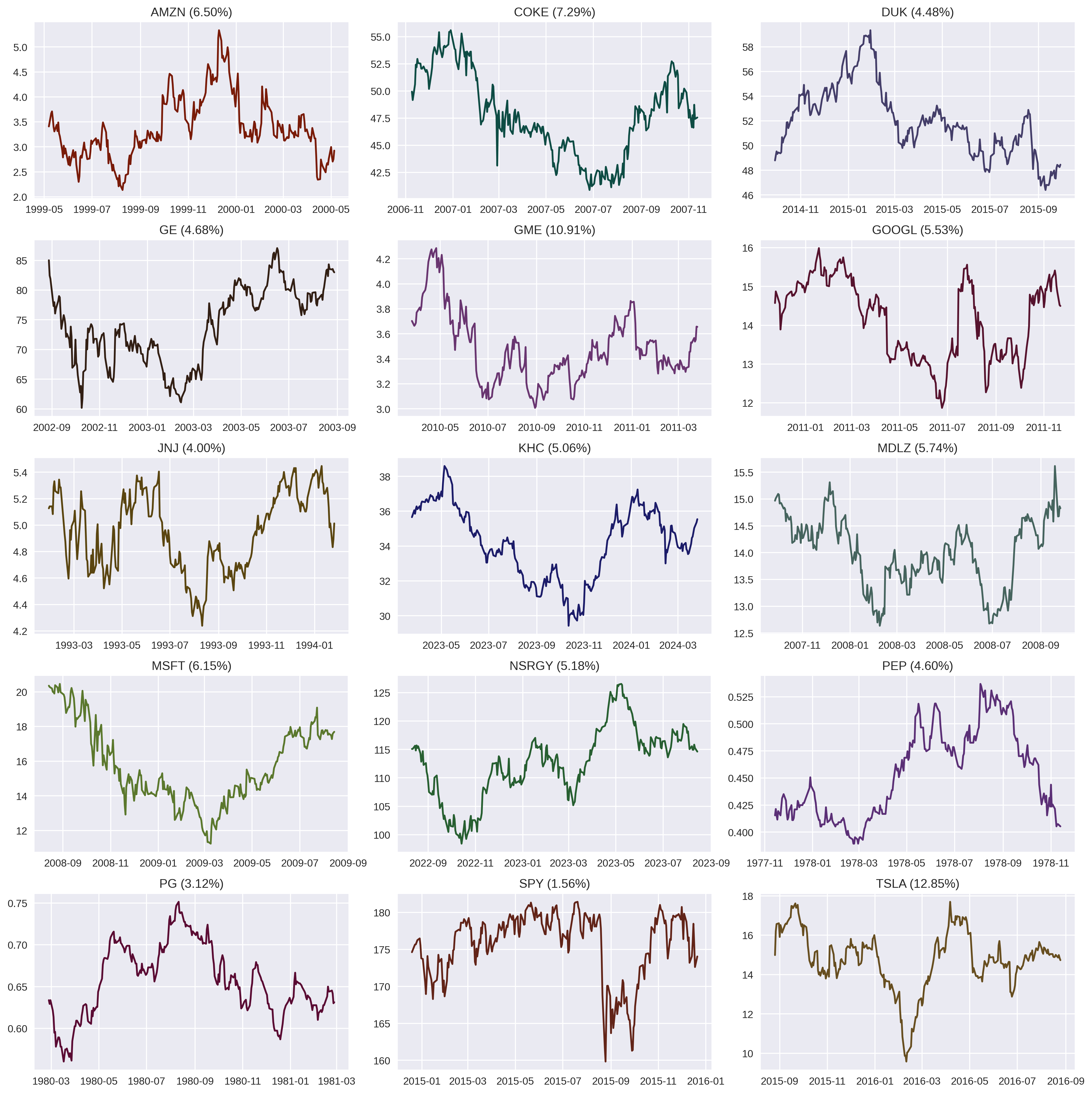
A smattering 15 stocks were chosen, and their mean daily returns were calculated over a sliding 252-day window. Random periods are plotted which have positive mean daily returns but negative total return across the period. Each ticker is displayed with its percentage of periods tested which have this characteristic.
Think about the implication:
-
An investor who buys the asset each morning and sells the following morning, while buying the asset again at the exact same price makes money.
-
An investor who buys and holds loses money.
This exercise also gives us a clue – more volatile stocks have a higher frequency of these pathological periods, and for any single stock, the periods occur during volatile periods. Whatever this thing is, it has something to do with volatility.
Indeed, this phenomenon is called volatility drag. To understand it better, we need to make a stop at the casino.
Great average returns do not a winner make
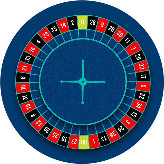
An American roulette table has 38 squares. Two squares are green, 18 are red, and 18 are black. The game starts by betting money on red or black. A ball is then spun around the wheel, randomly landing on a color. A correct guess doubles your money, and an incorrect guess loses the entire bet.
The expected winnings on a $1 bet is trivial to calculate:
Indeed, after games, the expected P&L is $.
So far so good. This is why no mathematicians play routlette. We can make roulette bets analogous to stock investing by simulating a single-period "buy and hold" strategy for some finite number of plays – we let our bet ride for rounds. Unsurprisingly, the expected final payout is abysmal:
But something quite interesting happens when we change the game slightly. Let’s imagine a roulette table which has inverted the odds in the gambler’s favor. At this table, the green squares are feebies - they always count as a win.
Now the expected return for a single play is positive.
Not only that, but the expected growth in wealth after plays is also positive, guaranteeing that the casino loses money in the long run.
Should we play this game?
We’ve just calculated the expected payout, but that number would only be realized after a sufficiently large number of -round plays. We might also wonder about the expected outcome of a single play. Because individual rounds multiply the starting wealth, the order doesn’t matter. Thus, the final wealth is fully determined by the number of wins. Each win occurs with probability , so the expected number of wins in an -round play is simply
Then the final return for a game which has the expected number of wins is
Therefore, it’s most likely that you will walk away with nothing each time you sit down to play! Sure, you could walk out the door with $ after 10 rounds, but that happens only with a chance! On the other hand, if you play a 10-round game 400 times, it’s more likely than not that you’ll have won $ at some point, only sacrificing $399 for the privilege.
We can also see a cartoon example of someone with positive average returns who still ends up a loser. Consider the unlucky soul who won 9 times in a row and lost on their 10th play. Their average return was a whopping 80% per play!
But of course, they ended up with a total return of -100%. The bigger the rise, the harder the fall.
Whether or not you would take this bet given finite money (i.e. finite number of plays) depends on your level of risk tolerance.
This is a variation on the St. Petersburg Paradox, which highlights the difference between the mathematical value of a game and a rational individual’s willingness to play it. This topic was also explored in a similar setting to this one by Paul Samuelson in 1971 (Samuelson (1971)).
Now, take a look at the quantity . Taking the log of both sides of the above equation,
This is the log return!
To summarize,
-
Simple returns tell us about the dynamics of the expected value of the price across many possible realizations of the path.
-
Log returns tell us about the dynamics of the expected path that the asset price takes.
This tracks with our discussion about the SPY time series. By accepting that time series data as our sample and declaring that it perfectly models the population statistics, we are not saying that "this sample has the mean growth rate;" rather, we are saying that "this sample has the most likely growth rate."
So, we’ve tracked down the difference in these two growth rates, but we’ll get a better feel for the machinery by building a bridge between the stock price and the casino. So far we’ve only been concerned with the first moment of our random returns, but in order to develop our model, we need to consider the second moment as well.
The binomial model
The binomial model provides the perfect setting for a random walk. It simplifies the math while providing some key ingredients:
-
a natural structure for geometric growth
-
sufficient degrees of freedom to tune distributions to our liking
-
in the limit, converges on Geometric Brownian Motion
A geometric version of the binomial model was introduced by Cox, Ross, and Rubinstein (1979) in 1979 to price options. I’ll refer to it as the Geometric Binomial Random Walk (GBRW). They also demonstrated that this option pricing method converges on the Black-Scholes-Merton solution. We won’t be pricing options here, but we’ll use a similar convergence technique to study and extend our stock price model.

In the GBRW model, the asset price rises to with probability or falls to in a single time step.
This is simply a generalization of the Roulette game from above.
One time step is not enough for our needs – we need to develop a procedure for extending the model to time scales larger and smaller than so we can examine the statistics2.
We begin by examining a simpler case: the Arithmetic Binomial Random Walk (ABRW).
Arithmetic binomial random walk
The arithmetic binomial random walk is characterized by step sizes that do not change with position or time. Here, I’ve kept the model general by allowing for asymmetric step sizes and probabilities.

There are many ways to frame and study this setting mathematically, but as a computer scientist by trade, I like the framing that facilitates simulation (i.e. one that allows repeated sampling). As it turns out, this approach also builds a nice bridge to stochastic calculus.
We will analyze the binomial model via the properties of a random walk along its tree-like structure. The engine of the random walk is the random variable .
This is already enough setup to do some interesting math, but the real meat comes from extending the definition of our model.
We recognize that daily returns for assets do not tell the full story. Rather, they are a snapshot at a resolution of . Thus, daily returns (simple or log) cannot be the atomic random variables! Just like how annual return is a random quantity constructed from random daily returns, so too are daily returns merely a summary of higher frequency trading. In the limit, we consider trading to occur continuously.
Therefore, in order for the binomial model to be useful to us, we need to be able to reason about its properties at time scales both larger and smaller than the timescale over which it is initially defined.
I like to think of it this way: by defining the sample space and probability measure at a particular time horizon, what we’re really doing is setting the parameters of a distribution at that time horizon. Then, we analyze the properties of the model at discrete interval lengths to find a continuous map from time to the distribution.
Think of as the resolution of the grid. It is the mesh of the partition of the time axis.
Now, consider the process
The logarithm turns the geometric binomial grid above into an arithmetic one.
Equivalently, one could also consider the random variable to be the number of up-moves, analogous to the number of wins in the Roulette example. Across one timestep, this is a boolean random variable.
At this point, the grid is only defined for times . So we look at how the expectation and variance evolve for . It’s relatively easy to work this out using the binomial distribution, or you can simply recognize that we are accumulating independent Bernoulli trials.
Because the quantities and are invariant for any , this gives us a natural procedure to extend the binomial grid definition to times between and ; i.e. to increase the resolution: iteratively partition the interval while preserving these two invariants3.
With this framing in mind, we’ll indicate the hard-coded parameters for the -resolution grid by defining constants.
We did a similar substitution at the beginning of this essay for the SPY time series. But in this case, the substitution results directly from how we’ve defined the binomial grid, not an emperical observation like before. Writing is useful because later on we will manipulate like a variable. It is justified because, as shown above, is linear in time, insofar as you consider a discrete function of time:
This essentially recognizes and as growth and volatility per unit time of respectively.
If the goal is to simulate a random walk on the binomial grid (e.g. with a computer), all we really need is a formula for the binomial random variable from which to sample to construct a random walk with timesteps of arbitrary length. We simply extend to , and define . Let
Then, we can simply increase until we have sufficient precision.
These two constraints in two unknowns gives a unique solution (up to a reflection about the first moment):
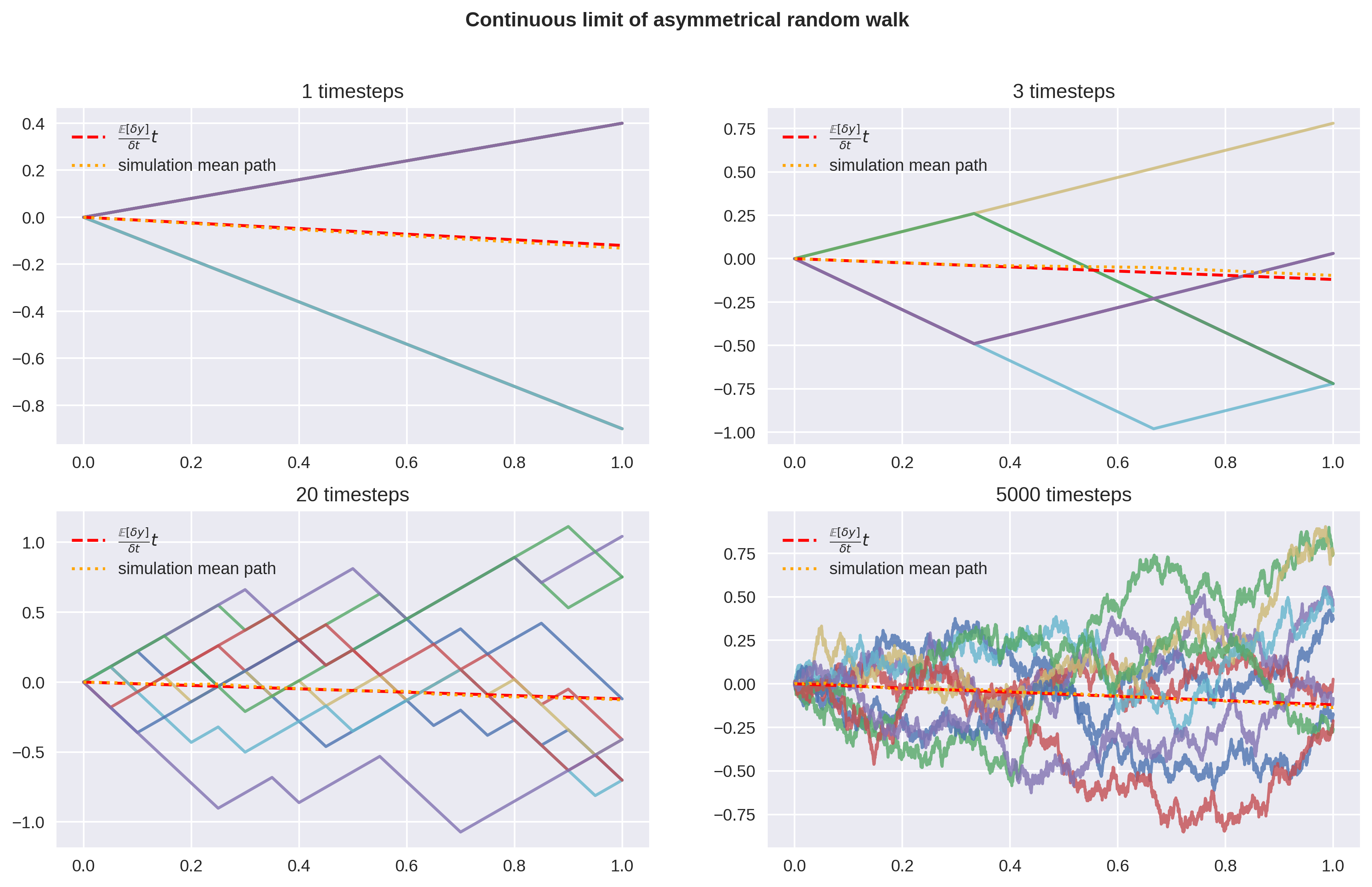
Here I’ve defined a linear binomial model by , , . The expected value and variance at time are invariant as the resolution of the binomial grid increases. is set to 1 w.l.o.g., and the mean path is interpolated to make the graph easier to read. The expectation of is linear in time.
What’s more, we can let become large, and with a healthy bit of applied math hand-waving, let
Voilà! We’ve discovered Brownian motion and stochastic increments!
It should be clear that we aren’t in Kansas anymore, and that normal rules of calculus don’t apply here. In traditional calculus, a differential is defined as the linear component of its function’s derivative:
But at no point (including in the limit) is differentiable!
Here we’ve approached through a limiting process of smaller and more frequent Bernoulli trials, so takes the form of a Bernoulli random variable. The more common (functionally equivalent) form is to write as a Gaussian random variable.
with .
All that’s left to do is integrate and exponentiate to obtain our simulated path.
Geometric binomial random walk
Now let’s find out what happens when we apply the same procedure for the geometric case.

Start by choosing a random variable which drives the random walker across the grid.
We would rather not have our random variable depend on (via , such that its distribution changes after each trial), so instead, we express the problem geometrically.
Whether you consider , itself, or even a growth factor like
to be the random variable, it makes no difference.
The key characteristic is that we are sampling an independent sequence of binomial random variables and accumulating them geometrically to walk along the binomial tree. These forms are all equivalent and lead to the same results below. Using or makes the math a bit cleaner (we don’t get popping up everywhere).
The expectation and variance across are
Because these values are just constants, we’ll write them as such.
Again, we write them this way to create quantities and which are expressed per unit time in anticipation of scaling the time interval of our trials later on. But at this point, is just a number, not a variable!
The next step is to find the first and second moments of the derived random variable, . Recall from the linear example that the goal is to establish a relationship between and which can be extended to all values of .
Across timesteps of length , the expectation is binomial.
This also follows from the expectation of independent variates.
This confirms that the expected total growth and thus the expected value of grows exponentially, which is unsurprising.
The variance isn’t quite as clean:
Nonetheless, we have the necessary formulae to determine our binomial random variables for any grid resolution. Again, extend to , with .
Since becomes small, we can simplify.
Now we notice something very interesting. Just like in the linear case, we have the scaling of the random variables proportional to . But instead of the and which describe the final distribution, we have new quantities.
What’s more, we can see that these values represent an expected value and variance of some other distribution on the time scale.
What are these spooky quantities? One option here is to recall that we ignore anything smaller than , in which case we simply have
But recall that by definition, at any grid resolution,
Thus,
This is our log return, corrected for convexity! I’ll spare the reader of the algebra, but the variance works out to
We’ve played fast and loose with our approximations here, so it’s worth taking a beat to notice that the growth and volatility densities and depend on , the starting resolution of the grid. This was not the case for and from the arithmetic binomial grid. In other words, in the process of refining the grid above, we swapped out for and for , but only at the resolution. This means that the error introduced at the resolution doesn’t vanish for smaller resolutions, so and should be sufficiently small.
In the limit, when and are Gaussian, these equations are exact:
Similarly, for the variance:
Once again, let’s consolidate the random variable and write its equivalent stochastic differential equation form:
Visualization
The arithmetic and geometric approach are equivalent at each resolution (to a close approximation).
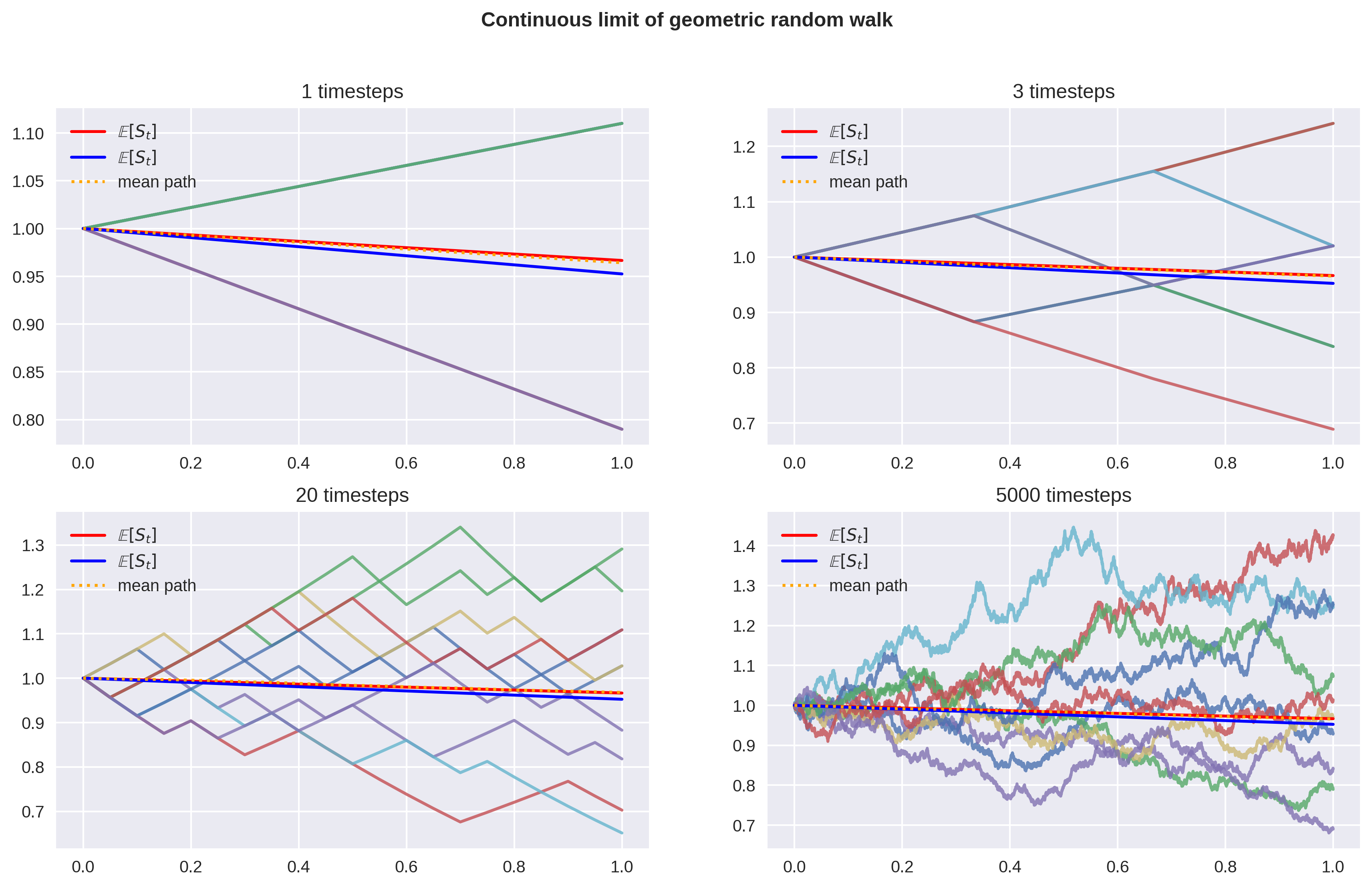
Here I’ve defined a geometric binomial model by , , . is set to 1 w.l.o.g., and the mean path is interpolated to make the graph easier to read. The expectation of is exponential in time.
Another view, for good measure:
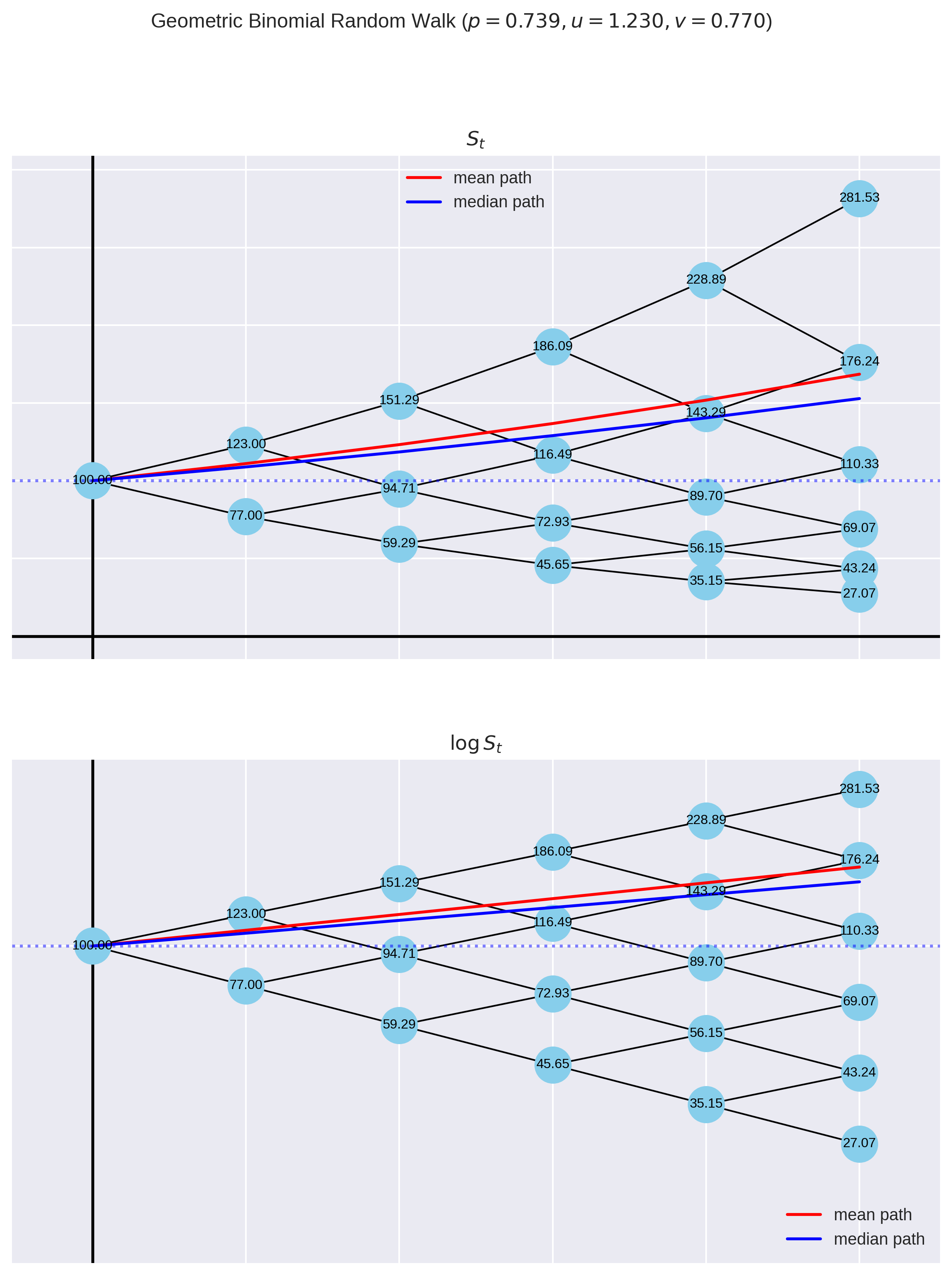
Here, I’ve used more human-friendly numbers that show a plausible stock price path over a few years. Volatility drag is the difference between mean and median paths taken through the binomial tree.
Conclusion - What a drag!
We have seen how the relationship between geometric growth and randomness leads to the phenomenon of volatility drag:
It can be described in many different, yet equivalent ways:
-
the difference between expected simple and log returns at any time scale
-
the convexity correction for exponential growth
-
the difference in growth between the mean price path and the median price path
-
the difference between arithmetic and geometric mean of growth rates
-
minus half the quadratic variation of
Bear in mind that simple vs log returns has nothing to do with "compounding," as I have seen claimed online.
All geometric (exponential) growth compounds, by definition.
Practitioners often model asset prices as Geometric Brownian Motion (if only as a precursor to more sophistocated methods) and sample historical price data at a particular resolution in order to estimate the parameters and for e.g. Monte Carlo simulations. As was stated earlier in this essay, by declaring that the historical (discrete!) time series data is representative of the population, we implicitly declare that our sample path grows at the median rate, not the mean rate!
There’s just one more loose end to tie up. If volatility drag is a negative correction, why did the analysis from the binomial model section end up with a positive correction, ? Most online materials and papers write Geometric Brownian Motion in terms of increments in (as opposed to increments in ).
Indeed, the and in this equation should be the simple return growth rate and volatility! In the notation used in this essay, the correct formula is
It is a common mistake to use the log return growth and volatility in this equation. I believe the mistake comes from the habit of working with log returns by default due to their nice properties, and failing to correct the quantities when plugging them into this most common GBM form.
I do wonder if there’s any money to be made in the market by arbitraging this bug which is no doubt running in some trading algorithm in some hedge fund somewhere, but the errors introduced by assuming Gaussian returns and assuming historical returns are predictive of future returns probably far outweighs the upside.
Additionally, in the Black-Scholes framework, the whole point is to eliminate by hedging anyways. This has the effect of setting the portfolio growth rate to , the continuously compounded risk-free rate. But of course, rates are quoted in simple terms, not log terms! That’s why, under the risk-neutral measure, the solution for applies the convexity correction downwards:
The same correction is seen in the solution to the Black-Scholes differential equation for call options.
References
Bachelier, Louis. 1900. “Théorie de La Spéculation.” Annales Scientifiques de L’Ecole Normale Supérieure 17: 21–88.
Cox, John C., Stephen A. Ross, and Mark Rubinstein. 1979. “Option Pricing: A Simplified Approach.” Journal of Financial Economics 7 (3): 229–63. https://doi.org/https://doi.org/10.1016/0304-405X(79)90015-1.
Samuelson, Paul A. 1971. “The "Fallacy" of Maximizing the Geometric Mean in Long Sequences of Investing or Gambling.” Proceedings of the National Academy of Sciences of the United States of America 68 (10): 2493–96. http://www.jstor.org/stable/61075.