Neural Networks from Scratch
Published May 18, 2024
Bootstrapping a mathematical and programmatic description of Neural Networks
Introduction
There are many great online resources for learning about neural networks. However, the recent fashionability of neural nets has seen a proliferation of introductory materials which mostly repackage the same few ideas. Search engines love the broad appeal of these blog posts and articles, but technically inclined readers are often left without the necessary intuitions that are required to build and operate these networks.
Fortunately, for such a powerful tool, Feedforward Neural Networks are relatively simple objects, the mechanics of which are digestible by those with a working knowledge of vector calculus and linear algebra.
The complexity of the study of networks as universal approximators comes when trying to prove statements about their expressivity and trainability, but these topics are not explored here.
In this essay, my goal is to build the core concepts of FNNs from the ground up while filling in some oft-missed details from other popular educational materials. To that end, this essay assumes the following of the reader.
-
Comfort with linear maps between real vector spaces and their matrix representations
-
Familiarity with multivariate calculus
-
Familiarity with the basic structure of a neural network
I would not publish this essay unless I thought I was bringing something new to the table; herein you will find the following:
-
An intuitive bridge between the index and vector interpretation of backpropagation
-
Preciseness / rigor preferred over notational simplicity
-
Special attention given to pitfalls on the way to building intuition
-
Intuition checks which I have not found elsewhere online
Please email any questions or feedback to brendan.schlaman@gmail.com.
Enjoy!
Heteroassociative memory and Hebb's Rule
Linear models such as linear associators are a critical building block in understanding neural networks, not only for their role in stitching together layers in a network, but also for their ability to store relationships.
Perhaps the simplest type of linear model is associative memory (content-addressable memory). Associators map arbitrary input representations to arbitrary output representations. We will focus on heteroassociative memory, which is used to retrieve patterns which differ (e.g. in encoding, dimensionality) from the input pattern, in contrast to autoassociative memory, used for pattern correction.
A theory for synaptic placticity was introduced by Donald Hebb in 1949, which showed how simple interactions between neurons can eventually learn information. The mathematical formulation of these ideas is called Hebbian learning, and it is a natural starting point for constructing a heteroassociative memory network.
A word of caution on an oft repeated falsehood: while it is indeed true that neurons of a human brain provided inspiration for elementary linear models, there is little in common between how modern neural nets learn and how humans learn!
The simple linear associator
The canonical application of Hebbian learning is the simple linear associator. It is a linear map from independent inputs to targets .
where and are matrices comprising the input and target patterns and respectively, arranged as columns. denotes the model's output (which may or may not match the desired targets ). The system learns by identifying a weight matrix which stores information about the associations between inputs and targets such that recall looks like a linear transformation from input to target space.
This type of "learning" is something of a toy, but it should convince you that information can be stored in weights between neurons, and indeed, requiring less space than rote memorization.
As we will see, perfect recall can be achieved under certain special conditions.
One-shot Hebbian learning (correlation memory)
Simple linear associators can be trained in one shot using Hebb's Rule by constructing a correlation matrix of the inputs and targets. Each entry in represents the correlation between an input and output neuron across datapoints.
Retrieval from a linear correlation memory reveals its limitations:
Two strict requirements are required for perfect retrieval:
-
must be normalized such that the term is 1 (or retrieval can be altered to divide by magnitude of the input).
-
The must be pairwise orthogonal such that the "cross-talk" terms are 0.
If these conditions are met, perfect retrieval after a single round of training is easy to prove. Suppose we are given a set of inputs and target values .
This follows from the fact orthonormal matrices have an inverse equal to their transpose.
Storage analysis
The orthogonality restriction greatly reduces the capacity of this memory. However, there are indeed theoretical savings to be had here. If tasked with storing an arbitrary linear map , one might naively record the inputs and outputs, requiring storage space for and 1. Encoding the map as a Simple Linear Associator requires only , the size of .
Generalization: on-line Hebbian learning
The above one-shot Hebbian learning rule can be generalized to accept inputs at different times, and indeed, in continuous time.
where denotes an outer product.
Hebbian on-line supervised learning:
The storage capacity for this associator is the same; only input-output pairs can be memorized at any given time, but here, pairs can be unlearned or reassigned at will.
Hebbian learning: a closer look
Consider a single iteration of online Hebbian learning with orthogonal inputs. That is, imagine after being presented with the th input / output pair, . is then an inner product:
In index notation, . The th row of can be interpreted as the input scaled by the output . Thus, during recall (let ), the are obtained by projecting onto each of these scaled input vectors, yielding the original (recall ).
This should make it clear why perfect recall requires that the be orthonormal. Orthonormal means that the rows of will be orthogonal, such that during recall, there will be no "crosstalk" or "interference" from other inputs.
Key takeaway:
The memory mechanism of Hebbian learning can be viewed as storing
scaled versions of of the input as the rows of , and
layering these orthogonal vectors using vector addition.
Beyond Hebb: the Delta Rule (Widrow-Hoff)
The orthonormality requirement for inputs above can be relaxed to a less restrictive linear independence requirement by introducing a new strategy for learning: the delta rule.
Widrow-Hoff is multiple linear regression
Analogy:
-
Each element of the target vector for i/o pair is analogous to a to-be-predicted observation
-
prediction variables are analogous to input vectors
-
regression coefficients correspond to a row in weight matrix
-
intercept corresponds to the bias oft assumed for the units.
-
the delta rule converges to the form which is analogous to lin reg:
Again, we wish to attain perfect recall of inputs . One might assume that, much like in the case of Hebbian learning with orthogonal inputs, the system can be solved with matrix inversion:
Interestingly this appears to be the exact form for the unique solution of a multi-linear regression extimator. But there is a subtle catch! In a linear regression setting, this only works if the feature vectors are linearly independent; in other words, the system must be overdetermined. This allows the Gram matrix to be inverted (recall that, by convention, the columns of are the features in linear regression).
By contrast, in a linear association context, an underdetermined system is required to enable perfect recall. Thus, unfortunately, is not invertible, and so the above procedure will not work.
One way to get around this limitation is to purposefully remove information from the inputs by trucating such that it's number of rows equal the number of pairs which must be perfectly recalled. This is equivalent to padding with 0s, representing a neural network that shuts off the signal from these redundant input neurons.
For the following, we can simplify the analysis by noticing that each of the output nodes (equivalently, the rows of ) can be viewed as completely separate problems, since they are independent. Focusing on a single , we want
If we attempted to proceed as above with a multiplicative update rule like Hebbian learning, the problem becomes clear.
An additional error term emerges, which in the Hebbian learning context, would represent the correlation between input examples.
Think about it this way: Unless the set of all previous are known, it is impossible to know which direction to extend so that it can recall . How can be updated in a way that interferes as little as possible with the already-stored pairs?
An update must incorporate information about the associations which have already been seen. One cannot update along an input without interfering with the stored memory.
The goal is to recall datapoints:
Going forward, I will drop the index, as we will focus on a single output. The independence of output nodes in a simple linear model means that the analysis generalizes trivially to all outputs.
When first approaching this topic, I wondered if it were possible to exploit the degrees of freedom in the weights to recover on-line Hebbian learning by performing a quasi-Gram-Schmidt routine on the , thus iteratively building up an orthonormal basis.
Start with .
Then, each successive update must satisfy the following constraints:
-
It is orthogonal to all previous .
-
recalls .
In practice this might look like
where are scalars which can be found algebraically at each step, and is the projection of onto .
This method works by constructing an orthonormal basis of which transforms the non-orthonormal into a pattern basis before once again transforming it to the output space. This is essentially equivalent to -decomposition.
However, this method is disadvantageous, as it requires retaining information about the components of as the algorithm progresses.
A key idea to unlocking a new approach to this problem was provided by Widrow and Hoff (1960) in 1960.
The Widrow-Hoff algorithm or delta rule is an incredibly powerful technique and a critical stop on our journey towards neural networks.
The quintessential optimization method for neural networks, gradient descent, simplifies to Widrow-Hoff for single-layer networks like linear associators.
It turns the search for into an optimization problem by introducing a notion of measurable error (which I will suggestively call ) for a single association pair:
Thus, the update to is made in the direction that yields the best reduction in error for that pair:
Unsurprisingly, the update is made in the direction of . While it would indeed be possible to update in one shot such that it recalls perfectly, notice that updating may increase the error for other input pairs, proportional to their correlation with . Instead, input / output pairs are repeatedly presented to the network until perfect convergence is achieved.
Another advantage of this method is that it is useful even in contexts when perfect recall is not possible; i.e. when the system is overdetermined. In that context, Widrow-Hoff is equivalent to online linear regression (i.e. gradient descent on linear regression)!
Linear models: conclusion
Now that the "learning" mechanism of the linear neural network has been demonstrated, what is actually being learned here?
The following analysis comes from the landmark book Parallel Distributed Processing (David E. Rumelhart, McClelland, and Group (1986)) and is my favorite result regarding linear associators.
Consider the recall procedure.
Before performing delta rule learning, we can reconceptualize the problem from neuron space into pattern space. Instead of a single transformation, we can think of recall as a 3 step process.
-
Convert the input neuron space into input pattern space
-
Map inputs patterns to outputs patterns
-
Convert the output pattern space into output neuron space
Summarizing,
Let's apply this to the delta rule.
The matrix is simply the correlation structure among the input examples; i.e. .
The learning process for and are equivalent at each step even though translating between them is not possible without full knowledge of the input patterns. In other words, can be considered a "hidden" parameter which influences how the training converges (i.e. the respective rates for different inputs). Even the outputs don't affect learning; they are completely independent! In other words, the difference in output activations for two given inputs is irrelevant; it is only the correlation of the inputs that affects the system's ability to learn the associations!
Notice, however, that , , and are common across all association problems of examples. The pattern basis is always the same, with converging on in the case where inputs are linearly independent. This means that the only information distinguishing one delta rule learning system from another is the correlations between inputs! This correlation alone scales the updates to and determines how the system converges.
The error found in the output pattern space for a given input can be interpreted as the degree to which the outputs of correlated features have not yet been corrected for by . The scaling of this error by highlights how highly correlated pairs will produce greater errors by weight at each step.
Another insight to notice here is that any modifications to the inputs which preserves their correlations will not be detected by the system.
Key insight:
This means that, in linear networks, the correlation among inputs is the
only thing that matters, even if the inputs and outputs are drawn from a
distribution. There is no hidden representation of knowledge which
associates inputs and outputs.
Important insight:
By introducing a measure of "distance" between the target and the
output, we can actually measure how good a prediction is and take steps
to making it better.
This is an additional layer beyond random pattern mapping, and it means we can still find decent solutions even when the inputs are linearly dependent (which is guaranteed to be the case if we have more pairs than we have input nodes). I would wager that the min error is better when similar inputs map to similar outputs, but I haven't proven this yet.
But this is interesting, from the book:
In a linear system, it is only the "structure" of the inputs and outputs that matter, not details of the internal representation of the system. It is only the pattern of correlations among the patterns that matter, not the contents of the specific patterns themselves.
For an overview of how associators behave in statistical environments, i.e. when the input output pairs are sampled from a distribution, I recommend reading Chapter 11 of Parallel Distributed Processing, Volume 1 written by G. O. Stone (David E. Rumelhart, McClelland, and Group (1986)[Chapter 11]).
Nonlinear models
It is a well known result that a network with consecutive linear layers (i.e. no activation) is equivalent to a network with a single layer (this is easy to prove and a worthwhile exercise). Thus, if we wish to broaden the space of learnable functions for network models, we must introduce nonlinearity into the system. In the simplest cases, this is done by applying nonlinear "activation" functions to the output neurons of a linear model.
The canonical instance of this type of architecture is the single-layer Perceptron (with outputs), often introduced as a nonlinear successor to linear models. However, I consider it somewhat tangent to the study of feedforward neural networks. The Perceptron convergence theorem is worth reviewing, but the algorithm itself applies only to a narrow class of problems. It is better suited as a precursor to Support Vector Machines.
A slightly more useful example of single layer, nonlinear network is the Bidirectional Associative Memory introduced by Bart Kosko in 1988 (Kosko (1988)). This is a natural extension of the associative memory discussed in the previous section, so I will explore it briefly here.
Bidirectional associative memories
The memory of linear associators can be improved by introducing nonlinearity and relaxing the perfect recall requirement.
Let and be bipolar vectors so as to increase the chances of inputs / outputs being orthogonal, and introduce the nonlinear operator to retrieval.
This association is bidirectional:
Here, the cross-talk term need only be small for perfect recall. The performance of this associator is inversely related to the pairwise correlation of the ; that is, the model has a hard time distinguishing between highly correlated inputs.
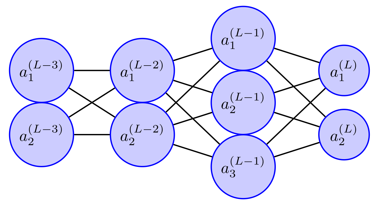
Feedforward Neural Networks (Multilayer Perceptrons)
The key difference between the class of models discussed up to this point and the class of models going forward is the introduction of hidden layers. In fact, calling linear associators "models" gives them too much credit - associators learn via rote memorization. They memorize geometric differences between inputs which are later recited. These associators only have enough degrees of freedom to intepret inputs as directions in -dimensional space, and thus perform terribly at simple tasks which require a more nuanced view of the inputs (encoding, bitwise operations, arithmetic operations, the XOR problem, etc).
Hidden layers allow for learning representations, which awards a massive step-up in the power to these models. I confess that I haven't yet found a particularly instructive bridge between associative networks and hidden layer networks. Perhaps this shouldn't be so surprising, as the evolution between the two paradigms took place over the better part of two decades. One possible angle to consider is that the Delta Rule is essentially a special case of gradient descent (on mean squared error loss function). But this conceptual discontinuity does not prevent us from adapting some of the language and mathematical formulations from our linear beginnings to this new setting. I may revisit this topic in the future. For now, we will explore the power of hidden layer architectures with fresh eyes.
One of the simplest kinds of hidden layer networks is the Feedforward Neural Network (FNN), sometimes called the multilayer Perceptron. Don't let the naming fool you - the multilayer Perceptron has little in common with the single-layer Perceptron because hidden layers change the whole game.
Ultimately, feedforward networks approximate some function by computing the function
where .
Notation
Getting the notation right is important for FNNs, and in this section, I will sacrifice brevity for precision at every turn. This section borrows some notation from Guilhoto (2018) and adds extra details which will prove useful.
I will use the following notation:
| Expression | Definition |
|---|---|
| The weights matrix comprising the weights that act on activated neurons. is an matrix, where is the width of layer , and is the width of layer . | |
| th row vector of . | |
| th column vector of . | |
| Element of . The weight of the connection of the th neuron of the th layer to the th neuron of the th layer. | |
| In general, will index the training examples, and and will index the rows and columns of various matrices respectively. will index the layer of the network, with being the final (output) layer. Layer can be interpreted as "owning" the weights which feed into it. Therefore, it is natural that indexes objects corresponding to neurons at this layer (e.g. activations , preactivations ). | |
| The activation function. For simplicity, we will assume that a single activation function is shared by the entire network. | |
| The output of the network at the final layer . This is the estimation. |
The astute reader will notice that I've almost completely omitted analysis of the bias term from this essay. This is quite intentional, as I don't believe it contributes much to the intuitions I'm looking to build here. There are plenty of other resources which provide the derivatives.
I don't want to list out the part of the engine. I want to show how it makes its power.
Review: FNN basics
The weighted sum of inputs to a layer can be interpreted as an affine transformation between real vector spaces.
Unlike in the linear context, however, the interpretation of this map is less straightforward. It may be useful to view the purpose of this transformation as enhancing the expressivity of the neural network. Dense layers vastly increase the searchable space of models and increase the generality of the architecture.
Despite great attention given to the weights in the linear models earlier in this essay, going forward, it may be prudent to avoid thinking too much about the weights in isolation. Rather, they are an efficient way to construct complicated functions with lots of parameters that possess important symmetries which can be exploited. The killer feature of neural networks is that we can repurpose both the mathematical and computational tools of linear algebra to manipulate state and train the network, providing an abundance of paths in parameter space to encode complex internal representations and dodge local minima as it searches through function space.
The layers in a NN act as a synchronization mechanism, meaning that layer nodes are activated at the same time. This gives the structure of the ensemble approximation function a natural composition, which is easy to deal with mathematically.
In fact, none of the results below require that layers be dense; connections may be omitted entirely or connect nonconsecutive layers.
That being said, it is true that the weights matrices (and the weights matrices alone) contain all information which a neural network has ever learned and (in the simplest case) deterministically decides its future performance. If AI bots become sentient, it will mean that tables of 64-bit floating point numbers are a suitable substrate in which an internal representation of conciousness itself can be embedded.
Forward pass notation
The linear transformation between dense layers is given by2
The activation of a single neuron (the th neuron of the th layer) is therefore
The contribution of the th layer to the th neuron of the th layer is:
The contribution of a single neuron (the th neuron of the th layer) to the th layer is:
where
I won't make much use of these equations, but it is worth understanding them as a description of the movement of data through the network.
Gradient descent and loss functions
Generally speaking, loss functions come in two broad flavors, the simplest cases of which will be described in this essay.
MSE incorporates both the variance of the estimator and its bias.
Gradient descent is a general numerical optimization method for finding function minimums which requires that updates to function parameters be in the opposite direction of that function's gradient:
There are many online resources which teach this method, so I won't rehash the topic here. I will, however, mention the one of the most important features of this method for our purposes: the gradient of a function is linear, and thus satisfies the additivity property:
This property allows us to aggregate gradients which were computed for different training examples independently.
Backpropagation
The real power of neural networks stems from their
-
symmetry (backwards looks a lot like forwards, layers synchronize per-neuron operations),
-
modularity (composable functions as independently-differentiable clusters), and
-
sparsity (linear map followed by element-wise activation)
embedded in their structure.
This section explains why densely connected networks are such a natural vehicle for performing gradient descent in high-dimensional parameter space. There are many other ways to construct complex models which, in theory, could be just as expressive and intelligent as neural networks (our own brains, for example!), but training them would be messy and slow.
Don't forget that all this flexibility comes at a cost. Training even the simplest multilayer network is np-complete (Blum and Rivest (1992)).
On vectorization and VJP
So far in this essay, I have not shied away from keeping notation and computations vectorized, and that will continue for this section. There are several reasons for this. For one, it is prudent to keep analysis of any system as general as possible for as long as possible such that tools built up in the process can be ported to other domains more easily, and so a greater catalog of optimizations remain applicable. In the case of the backpropagation algorithm, operation of networks via the language of vector calculus enables them to benefit from parallel computing and graphics libraries. Additionally, by putting in some work up front, we get input batching for free. Do not take this fact for granted! It is a beautiful consequence of linear algebra that we can pass stacks of independent data around in our networks without updating any of the mathematics or code.
That being said, one might wonder what makes FNNs such a hot commodity nowadays. The tabloid headline is that neural net architectures are the most flexible and efficient ways to optimize functions for a given level of expressivity3. No neurologist worth their salt would make the claim that the synapse chains in our brains behave anything like GPT-4. If the original neuronal approximators were inspired by biology, they certainly aren't anymore. The pictures of circles connected by lines which we draw for ourselves are, of course, merely representational4. CPUs move data between registers and perform simple arithmetic on the values they store - there is no grey matter hiding in your laptop.
That being said, there will be a trap waiting for us in the development of backprop if we simply close our eyes and let vector calculus take the wheel.
The tricky bit in the analysis of feedforward networks is that matrices are being used in two distinct ways:
-
as a linear subcomponent of the entire function; a transfer function between layers - a way to move data backwards and forwards through the network
-
as a means to enumerate paths of influence of the parameters (weights) during gradient computation - a way to store and chain derivatives along a compounding number of paths in the network
Great care should be taken to understand which case is in play in each moment, as the next example shows. In many introductory materials on neural networks, this inequivalence goes unaddressed.
The universality of the chain rule and the linear tools of vector calculus means that they are ignorant of the latent efficiencies available for exploit in the network. Following the letter of the law with these mathematical tools in the hopes of computing the perfect loss gradient leads to inefficient structures (order tensors, large Jacobians) which can be cleverly avoided.
Most introductory materials on this subject optimize prematurely in my view. I want to emphasize that naively throwing Jacobians at the problem is perfectly valid and has wonderful sanity checking mechanisms baked in. I encourage the reader to try this approach at least once and at least verify that the matrix dimensions really do match up.
With the preamble out of the way, what are these mysterious optimizations? They go by the name Vector Jacobian Product (VJP). The punchline is that in practice, no actual Jacobians need to be computed during gradient descent! It turns out that, due to the compute graph enforced by the network architecture, the product of any Jacobian with its neighboring vector in the derivative chain can be computed directly; i.e. without first computing the components of the product.
In some sense, this is the essence of Neural Networks, and I think it goes underappreciated.
Before jumping into VJP, let's trudge through the brute-force Jacobian approach. The chain rule tracks and merges the contributions of independent variables to the final outputs of a function along all possible paths of influence. Vector calculus accounts for these paths (to a linear approximation) by recording Cartesian products of intermediate variable dependencies in the form of first-order partial derivatives. By arranging these partial derivatives into a matrix (the Jacobian), the job of path enumeration and combinatorics can be offloaded to linear algebra. Any complicated variable dependency graph just looks like composed matrix multiplication! Consider the following linear transition from layer to layer :
Despite the transition being written in vector form, the chain rule as carried out via vector calculus sees this operation as
where is treated as a parameter of during derivative computation.
Watch out - is not the same as ! describes the parameters of the linear function , whereas is merely an alias for !
We might then write an network like so:
where , , represent arbitrary vector-valued functions which operate on inputs, somehow incorporating the weights. Then we would write the Jacobian of with respect to, for example, as
There is nothing inconsistent about this view of the system, and in fact, it is already quite good (if suboptimal); the intermediate derivatives like can be computed once and then reused for calculating all gradients which appear to its left in the network.
But we know something that the calculus doesn't! This is where differentiating between the two distinct applications of linear algebra is critical. To see where we might save CPU cycles, notice that only of the possible derivatives will be nonzero. This is because for a vanilla FNN, these intermediate transition functions between layers are constrained to be linear maps followed by nonlinear scalar functions applied element-wise.
VJP to the rescue:
-
For linear maps, VJP allows us to replace the Jacobian with the transpose of the weights matrix
-
For element-wise functions, VJP allows us to use Hadamard products
The Backprop Toolkit
The following results provide us with tools to aid in interpreting and simplifying notation later on while tackling the backpropagation algorithm.
Neuronal gradient symmetry
Recall the following from the definition of the forward-pass:
Dense, linear connections between layers leads to a nice result which provides a mechanism for propagating errors backwards through the network.
The consequence is that the exact same network can be used in reverse to compute gradients with no more difficulty than the forward pass. Ponder this for a moment. The ubiquity of neural networks owes a great debt to this special property.
Delta
As the error derivatives get passed back through the network, the intermediate quantities are somewhat analogous to the activated neurons at each layer.
is the celebrity VJP in backpropagation, but I reiterate that it is not strictly required to describe or implement backpropagation; it is nothing more than a location along the derivative chain where we've made a strategic substitution.
We will use it here, though, as it helps conceptualize the data flow during backpropagation and is emphasized in the literature (e.g. David E. Rumelhart, Hinton, and Williams (1986)).
It is also common to see this kind of notation (e.g. (Nielsen, n.d.)):
I tend to avoid this notation because it hides some subtle details while also importing operations which aren't actually needed. By avoiding the gradient operator (in favor of total derivatives and Jacobians), we can also avoid using the Hadamard product. This is because the Jacobian matrix is diagonal, which has the desired effect of element-wise multiplication.
Ultimately, I prefer the partial derivative notation because
-
the matrix dimensions provide for easy sanity checks, and
-
the technique generalizes better to other architectures (there is no magic - it's just the chain rule!)
During backpropagation, just as in the forward pass, the activations are computed based on previous activations, so it's useful to keep track of this relationship between the of subsequent layers.
Of course, can be recursively expanded to obtain a symbolic chain of derivatives.
Consider what happens to the quantity
when it is applied to the right-hand side of the above formula.
Starting at the end of the network and working backwards, for each layer, that numerical quantity is first sent backward to the previous layer by transforming it with the transpose of the weights matrix. It is then "activated" by scaling the components of the output by the derivative of the activation function at its inputs during the forward pass.
Note that this does not undo the forward pass, we are simply moving data in the reverse direction.
Generalized weights gradient
These "activated" and backpropagated intermediate sub-network derivatives can be accumulated such that only a single backward pass is required.
The formula for weight derivatives for a layer is simply
where the partial derivative for the biases is included for completeness. This should look familiar - it is the same as the delta update rule from the linear model section!
An apt summary of backprop from (Peter Bloem, n.d.):
We work out the derivatives of the parts symbolically, and then chain these together numerically.
Backpropagation algorithm
Now we can express the backpropagation algorithm in full. The below algorithm assumes that the preactivations and activations and the training example have been stored.
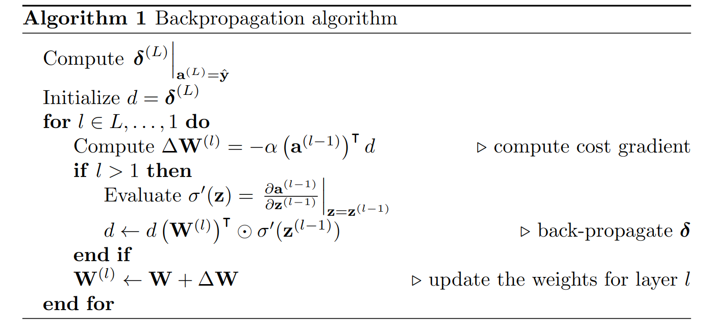
Note that in practice, the weights are often updated in a single shot at the end of the backward pass by some type of optimizer that modulates training parameters like learning rates and momentum. In the algorithm above, the weights are updated at each layer to emphasize the modularity of the updates.
References
Blum, Avrim L., and Ronald L. Rivest. 1992. "Training a 3-Node Neural Network Is NP-Complete." Neural Networks 5 (1): 117--27. https://doi.org/
Guilhoto, Leonardo Ferreira. 2018. "An Overview of Artificial Neural Networks for Mathematicians." In.
Kosko, B. 1988. "Bidirectional Associative Memories." IEEE Transactions on Systems, Man, and Cybernetics 18 (1): 49--60.
Nielsen, Michael. n.d. "Chapter 2: How the Backpropagation Algorithm Works."
Peter Bloem, Vrije Universiteit Amsterdam. n.d. "Backpropagation." .
Rumelhart, David E, Geoffrey E Hinton, and Ronald J Williams. 1986. "Learning Representations by Back-Propagating Errors." Nature 323: 533--36.
Rumelhart, David E., James L. McClelland, and PDP Research Group. 1986. Parallel Distributed Processing, Volume 1: Explorations in the Microstructure of Cognition: Foundations. The MIT Press.
Widrow, Bernard, and Marcian E. Hoff. 1960. "(1960) Bernard Widrow and Marcian E. Hoff, "Adaptive switching circuits," 1960 IRE WESCON Convention Record, New York: IRE, pp. 96-104." In Neurocomputing, Volume 1: Foundations of Research. The MIT Press.
-
Yes, yes, the orthonormality constraint on the inputs would allow one to compress this data quite a bit, but the Ordnung is still the same.↩
-
Modern machine learning frameworks typically use batch-major inputs, and it's conventional in computer science to think of the first dimension of e.g. a
tensor.Tensorobject as the rows of a matrix. Under this interpretation, the notation is reversed, and linear transformations look like -
It's quite difficult to formalize this statement; I may revisit this topic in the future.↩
-
How meta!↩